表格可视化#
本节演示如何使用 Styler 类进行表格数据的可视化。有关图表可视化的信息,请参阅 图表可视化。本文档以 Jupyter Notebook 形式编写,可在此处查看或下载。
Styler 对象和显示自定义#
样式和输出显示自定义应在 DataFrame 中的数据处理之后进行。如果 DataFrame 发生进一步更改,Styler 不会动态更新。DataFrame.style 属性是一个返回 Styler 对象的属性。它定义了 _repr_html_ 方法,因此它会在 Jupyter Notebook 中自动渲染。
Styler 主要设计用于小数据,但也可用于大数据,目前能够输出以下格式:
HTML
LaTeX
字符串(以及扩展的 CSV)
Excel
(JSON 目前不可用)
其中前三种格式具有设计用于格式化和自定义输出的显示自定义方法。这些方法包括:
使用 .format() 和 .format_index() 格式化值、索引和列标题,
使用 .relabel_index() 重命名索引或列标题标签,
使用 .hide() 隐藏某些列、索引和/或列标题,或索引名称,
使用 .concat() 拼接相似的 DataFrame。
格式化显示#
格式化值#
Styler 区分显示值和实际值,包括数据值以及索引或列标题。为了控制显示值,每个单元格中的文本都以字符串形式打印,我们可以使用 .format() 和 .format_index() 方法根据格式规范字符串或接受单个值并返回字符串的可调用对象来操作它。可以为整个表格或索引,或为单个列或 MultiIndex 级别定义此操作。我们还可以覆盖索引名称。
此外,格式化函数还具有一个 precision 参数,专门用于帮助格式化浮点数,以及 decimal 和 thousands 分隔符以支持其他区域设置,一个 na_rep 参数用于显示缺失数据,以及 escape 和 hyperlinks 参数用于帮助显示安全 HTML 或安全 LaTeX。默认格式化程序配置为采用 pandas 的全局选项,例如 styler.format.precision 选项,可通过 with pd.option_context('format.precision', 2): 控制。
[2]:
import pandas as pd
import numpy as np
import matplotlib as mpl

df = pd.DataFrame({
    "strings": ["Adam", "Mike"],
    "ints": [1, 3],
    "floats": [1.123, 1000.23]
})
df.style \
  .format(precision=3, thousands=".", decimal=",") \
  .format_index(str.upper, axis=1) \
  .relabel_index(["row 1", "row 2"], axis=0)
[2]:
| 字符串 | 整数 | 浮点数 | |
|---|---|---|---|
| 第 1 行 | 亚当 | 1 | 1,123 |
| 第 2 行 | 麦克 | 3 | 1.000,230 |
使用 Styler 操作显示是一个有用的功能,因为它维护索引和数据值用于其他目的,从而提供更大的控制。您无需为了按照自己的喜好显示 DataFrame 而覆盖它。这是一个更全面的示例,演示了如何在仍然依赖底层数据进行索引和计算的同时使用格式化函数。
[3]:
weather_df = pd.DataFrame(np.random.rand(10,2)*5,
                          index=pd.date_range(start="2021-01-01", periods=10),
                          columns=["Tokyo", "Beijing"])

def rain_condition(v):
    if v < 1.75:
        return "Dry"
    elif v < 2.75:
        return "Rain"
    return "Heavy Rain"

def make_pretty(styler):
    styler.set_caption("Weather Conditions")
    styler.format(rain_condition)
    styler.format_index(lambda v: v.strftime("%A"))
    styler.background_gradient(axis=None, vmin=1, vmax=5, cmap="YlGnBu")
    return styler

weather_df
[3]:
| 东京 | 北京 | |
|---|---|---|
| 2021-01-01 | 4.532926 | 0.152825 |
| 2021-01-02 | 2.077947 | 0.134430 |
| 2021-01-03 | 4.271864 | 4.629637 |
| 2021-01-04 | 0.453176 | 4.113319 |
| 2021-01-05 | 3.269600 | 3.838656 |
| 2021-01-06 | 1.138438 | 2.210950 |
| 2021-01-07 | 2.923515 | 1.835327 |
| 2021-01-08 | 0.563624 | 4.249480 |
| 2021-01-09 | 4.844616 | 0.582428 |
| 2021-01-10 | 1.061082 | 0.482518 |
[4]:
weather_df.loc["2021-01-04":"2021-01-08"].style.pipe(make_pretty)
[4]:
| 东京 | 北京 | |
|---|---|---|
| 星期一 | 干燥 | 大雨 |
| 星期二 | 大雨 | 大雨 |
| 星期三 | 干燥 | 雨 |
| 星期四 | 大雨 | 雨 |
| 星期五 | 干燥 | 大雨 |
隐藏数据#
索引和列标题可以完全隐藏,也可以选择性地排除某些行或列。这两种选项都使用相同的方法来实现。
通过不带任何参数调用 .hide() 可以隐藏索引,这在索引是基于整数时可能很有用。同样,通过不带任何进一步参数调用 .hide(axis=”columns”) 可以隐藏列标题。
可以通过调用相同的 .hide() 方法并将行/列标签、类似列表的对象或行/列标签的切片传递给 subset 参数来隐藏特定的行或列。
隐藏不会改变 CSS 类的整数排列,例如,隐藏 DataFrame 的前两列意味着列类索引仍将从 col2 开始,因为 col0 和 col1 只是被忽略了。
[5]:
df = pd.DataFrame(np.random.randn(5, 5))
df.style \
  .hide(subset=[0, 2, 4], axis=0) \
  .hide(subset=[0, 2, 4], axis=1)
[5]:
| 1 | 3 | |
|---|---|---|
| 1 | -0.529738 | 0.025776 |
| 3 | 0.056062 | 0.214816 |
要将此功能反转为显示功能,最好是组合一个隐藏项目的列表。
[6]:
show = [0, 2, 4]
df.style \
  .hide([row for row in df.index if row not in show], axis=0) \
  .hide([col for col in df.columns if col not in show], axis=1)
[6]:
| 0 | 2 | 4 | |
|---|---|---|---|
| 0 | 1.089193 | -0.737775 | 0.328942 |
| 2 | 1.350488 | 0.697516 | -0.395049 |
| 4 | -0.261027 | -0.226475 | 0.139844 |
拼接 DataFrame 输出#
只要它们共享相同的列,就可以将两个或更多个 Styler 拼接在一起。这对于显示 DataFrame 的汇总统计信息非常有用,并且通常与 DataFrame.agg 结合使用。
由于拼接的对象是 Styler,它们可以独立地进行样式设置,如下所示,并且它们的拼接会保留这些样式。
[7]:
summary_styler = df.agg(["sum", "mean"]).style \
                   .format(precision=3) \
                   .relabel_index(["Sum", "Average"])
df.style.format(precision=1).concat(summary_styler)
[7]:
| 0 | 1 | 2 | 3 | 4 | |
|---|---|---|---|---|---|
| 0 | 1.1 | 0.6 | -0.7 | 0.8 | 0.3 |
| 1 | -0.1 | -0.5 | -0.7 | 0.0 | 0.8 |
| 2 | 1.4 | 1.1 | 0.7 | -1.1 | -0.4 |
| 3 | -0.0 | 0.1 | 0.6 | 0.2 | 0.1 |
| 4 | -0.3 | -1.4 | -0.2 | 0.3 | 0.1 |
| 总和 | 2.004 | -0.087 | -0.295 | 0.264 | 0.948 |
| 平均值 | 0.401 | -0.017 | -0.059 | 0.053 | 0.190 |
Styler 对象和 HTML#
Styler 最初是为了支持广泛的 HTML 格式选项而构建的。其 HTML 输出会创建 HTML <table> 并利用 CSS 样式语言来操作许多参数,包括颜色、字体、边框、背景等。有关 HTML 表格样式的更多信息,请参阅此处。这提供了很大的开箱即用灵活性,甚至使网页开发者能够将 DataFrames 集成到他们现有的用户界面设计中。
下面我们演示默认输出,它看起来与标准 DataFrame HTML 表示非常相似。但是这里的 HTML 已经为每个单元格附加了一些 CSS 类,即使我们还没有创建任何样式。我们可以通过调用 .to_html() 方法来查看这些类,该方法将原始 HTML 作为字符串返回,这对于进一步处理或添加到文件中很有用——请继续阅读 有关 CSS 和 HTML 的更多信息。本节还将提供如何将此默认输出转换为更具表现力的 DataFrame 输出的演练。例如,我们如何构建 s
[8]:
df = pd.DataFrame([[38.0, 2.0, 18.0, 22.0, 21, np.nan],[19, 439, 6, 452, 226,232]],
                  index=pd.Index(['Tumour (Positive)', 'Non-Tumour (Negative)'], name='Actual Label:'),
                  columns=pd.MultiIndex.from_product([['Decision Tree', 'Regression', 'Random'],['Tumour', 'Non-Tumour']], names=['Model:', 'Predicted:']))
df.style
[8]:
| 模型 | 决策树 | 回归 | 随机 | |||
|---|---|---|---|---|---|---|
| 预测 | 肿瘤 | 非肿瘤 | 肿瘤 | 非肿瘤 | 肿瘤 | 非肿瘤 |
| 实际标签 | ||||||
| 肿瘤(阳性) | 38.000000 | 2.000000 | 18.000000 | 22.000000 | 21 | nan |
| 非肿瘤(阴性) | 19.000000 | 439.000000 | 6.000000 | 452.000000 | 226 | 232.000000 |
[10]:
s
[10]:
| 模型 | 决策树 | 回归 | ||
|---|---|---|---|---|
| 预测 | 肿瘤 | 非肿瘤 | 肿瘤 | 非肿瘤 |
| 实际标签 | ||||
| 肿瘤(阳性) | 38 | 2 | 18 | 22 |
| 非肿瘤(阴性) | 19 | 439 | 6 | 452 |
我们采取的第一步是从 DataFrame 创建 Styler 对象,然后通过使用 .hide() 隐藏不需要的列来选择感兴趣的范围。
[11]:
s = df.style.format('{:.0f}').hide([('Random', 'Tumour'), ('Random', 'Non-Tumour')], axis="columns")
s
[11]:
| 模型 | 决策树 | 回归 | ||
|---|---|---|---|---|
| 预测 | 肿瘤 | 非肿瘤 | 肿瘤 | 非肿瘤 |
| 实际标签 | ||||
| 肿瘤(阳性) | 38 | 2 | 18 | 22 |
| 非肿瘤(阴性) | 19 | 439 | 6 | 452 |
添加样式的方法#
为 Styler 添加自定义 CSS 样式有3 种主要方法:
使用 .set_table_styles() 控制表格的更广泛区域,并指定内部 CSS。虽然表格样式允许灵活添加 CSS 选择器和属性来控制表格的所有各个部分,但对于单个单元格的规范来说却显得笨拙。另请注意,表格样式无法导出到 Excel。
使用 .set_td_classes() 直接将外部 CSS 类链接到您的数据单元格,或链接由 .set_table_styles() 创建的内部 CSS 类。请参阅此处。这些方法不能用于列标题行或索引,也无法导出到 Excel。
使用 .apply() 和 .map() 函数为特定数据单元格添加直接内部 CSS。请参阅此处。自 v1.4.0 起,还有直接作用于列标题行或索引的方法;.apply_index() 和 .map_index()。请注意,只有这些方法添加的样式才能导出到 Excel。这些方法的工作方式与 DataFrame.apply() 和 DataFrame.map() 类似。
表格样式#
表格样式足够灵活,可以控制表格的所有单独部分,包括列标题和索引。但是,对于单个数据单元格或任何类型的条件格式,它们可能很难输入,因此我们建议将表格样式用于广泛的样式设置,例如一次性对整个行或列进行样式设置。
表格样式还用于控制可以一次性应用于整个表格的功能,例如创建通用的悬停功能。:hover 伪选择器以及其他伪选择器只能以这种方式使用。
为了复制 CSS 选择器和属性(属性值对)的常规格式,例如
tr:hover {
  background-color: #ffff99;
}
将样式传递给 .set_table_styles() 的必要格式是字典列表,每个字典都包含一个 CSS 选择器标签和 CSS 属性。属性可以是 2 元组列表,也可以是常规 CSS 字符串,例如
[13]:
cell_hover = {  # for row hover use <tr> instead of <td>
    'selector': 'td:hover',
    'props': [('background-color', '#ffffb3')]
}
index_names = {
    'selector': '.index_name',
    'props': 'font-style: italic; color: darkgrey; font-weight:normal;'
}
headers = {
    'selector': 'th:not(.index_name)',
    'props': 'background-color: #000066; color: white;'
}
s.set_table_styles([cell_hover, index_names, headers])
[13]:
| 模型 | 决策树 | 回归 | ||
|---|---|---|---|---|
| 预测 | 肿瘤 | 非肿瘤 | 肿瘤 | 非肿瘤 |
| 实际标签 | ||||
| 肿瘤(阳性) | 38 | 2 | 18 | 22 |
| 非肿瘤(阴性) | 19 | 439 | 6 | 452 |
接下来,我们再添加一些样式工件,以针对表格的特定部分。这里要小心,因为我们正在链式调用方法,我们需要明确指示该方法不要覆盖现有样式。
[15]:
s.set_table_styles([
    {'selector': 'th.col_heading', 'props': 'text-align: center;'},
    {'selector': 'th.col_heading.level0', 'props': 'font-size: 1.5em;'},
    {'selector': 'td', 'props': 'text-align: center; font-weight: bold;'},
], overwrite=False)
[15]:
| 模型 | 决策树 | 回归 | ||
|---|---|---|---|---|
| 预测 | 肿瘤 | 非肿瘤 | 肿瘤 | 非肿瘤 |
| 实际标签 | ||||
| 肿瘤(阳性) | 38 | 2 | 18 | 22 |
| 非肿瘤(阴性) | 19 | 439 | 6 | 452 |
作为便利方法(自版本 1.2.0 起),我们还可以将一个 dict 传递给 .set_table_styles(),其中包含行或列键。在后台,Styler 只是索引键并根据需要向给定的 CSS 选择器添加相关的 .col<m> 或 .row<n> 类。
[17]:
s.set_table_styles({
    ('Regression', 'Tumour'): [{'selector': 'th', 'props': 'border-left: 1px solid white'},
                               {'selector': 'td', 'props': 'border-left: 1px solid #000066'}]
}, overwrite=False, axis=0)
[17]:
| 模型 | 决策树 | 回归 | ||
|---|---|---|---|---|
| 预测 | 肿瘤 | 非肿瘤 | 肿瘤 | 非肿瘤 |
| 实际标签 | ||||
| 肿瘤(阳性) | 38 | 2 | 18 | 22 |
| 非肿瘤(阴性) | 19 | 439 | 6 | 452 |
设置类并链接到外部 CSS#
如果您已经设计了一个网站,那么您很可能已经有一个外部 CSS 文件来控制其中表格和单元格对象的样式。您可能希望使用这些原生文件,而不是在 Python 中复制所有 CSS(并复制任何维护工作)。
表格属性#
使用 .set_table_attributes() 可以非常轻松地向主 <table> 添加 class。此方法还可以附加内联样式——在 CSS 层级 中阅读更多信息。
[19]:
out = s.set_table_attributes('class="my-table-cls"').to_html()
print(out[out.find('<table'):][:109])
<table id="T_xyz01" class="my-table-cls">
  <thead>
    <tr>
      <th class="index_name level0" >Model:</th>
数据单元格 CSS 类#
版本 1.2.0 新增
.set_td_classes() 方法接受一个 DataFrame,其索引和列与底层 Styler 的 DataFrame 匹配。该 DataFrame 将包含字符串作为 CSS 类,以添加到各个数据单元格中:即 <table> 的 <td> 元素。我们不会使用外部 CSS,而是将在内部创建类并将其添加到表格样式中。我们将把添加边框的工作留到工具提示和标题部分。
[20]:
s.set_table_styles([  # create internal CSS classes
    {'selector': '.true', 'props': 'background-color: #e6ffe6;'},
    {'selector': '.false', 'props': 'background-color: #ffe6e6;'},
], overwrite=False)
cell_color = pd.DataFrame([['true ', 'false ', 'true ', 'false '],
                           ['false ', 'true ', 'false ', 'true ']],
                          index=df.index,
                          columns=df.columns[:4])
s.set_td_classes(cell_color)
[20]:
| 模型 | 决策树 | 回归 | ||
|---|---|---|---|---|
| 预测 | 肿瘤 | 非肿瘤 | 肿瘤 | 非肿瘤 |
| 实际标签 | ||||
| 肿瘤(阳性) | 38 | 2 | 18 | 22 |
| 非肿瘤(阴性) | 19 | 439 | 6 | 452 |
Styler 函数#
作用于数据#
我们使用以下方法来传递您的样式函数。这两种方法都接受一个函数(和一些其他关键字参数),并以特定方式将其应用于 DataFrame,从而渲染 CSS 样式。
.map() (逐元素):接受一个函数,该函数接受单个值并返回一个包含 CSS 属性-值对的字符串。
.apply()(按列/行/表):接受一个函数,该函数接受 Series 或 DataFrame 并返回具有相同形状的 Series、DataFrame 或 numpy 数组,其中每个元素都是一个包含 CSS 属性-值对的字符串。此方法一次传递 DataFrame 的每一列或每一行,或一次传递整个表,具体取决于
axis关键字参数。对于按列使用axis=0,按行使用axis=1,对于整个表一次性使用axis=None。
此方法对于将多个复杂逻辑应用于数据单元格非常强大。我们创建一个新的 DataFrame 来演示这一点。
[22]:
np.random.seed(0)
df2 = pd.DataFrame(np.random.randn(10,4), columns=['A','B','C','D'])
df2.style
[22]:
| A | B | C | D | |
|---|---|---|---|---|
| 0 | 1.764052 | 0.400157 | 0.978738 | 2.240893 |
| 1 | 1.867558 | -0.977278 | 0.950088 | -0.151357 |
| 2 | -0.103219 | 0.410599 | 0.144044 | 1.454274 |
| 3 | 0.761038 | 0.121675 | 0.443863 | 0.333674 |
| 4 | 1.494079 | -0.205158 | 0.313068 | -0.854096 |
| 5 | -2.552990 | 0.653619 | 0.864436 | -0.742165 |
| 6 | 2.269755 | -1.454366 | 0.045759 | -0.187184 |
| 7 | 1.532779 | 1.469359 | 0.154947 | 0.378163 |
| 8 | -0.887786 | -1.980796 | -0.347912 | 0.156349 |
| 9 | 1.230291 | 1.202380 | -0.387327 | -0.302303 |
例如,我们可以构建一个函数,如果文本为负数则将其着色,并将其与一个部分淡化可忽略值单元格的函数链式调用。由于这会依次查看每个元素,因此我们使用 map。
[23]:
def style_negative(v, props=''):
    return props if v < 0 else None
s2 = df2.style.map(style_negative, props='color:red;')\
              .map(lambda v: 'opacity: 20%;' if (v < 0.3) and (v > -0.3) else None)
s2
[23]:
| A | B | C | D | |
|---|---|---|---|---|
| 0 | 1.764052 | 0.400157 | 0.978738 | 2.240893 |
| 1 | 1.867558 | -0.977278 | 0.950088 | -0.151357 |
| 2 | -0.103219 | 0.410599 | 0.144044 | 1.454274 |
| 3 | 0.761038 | 0.121675 | 0.443863 | 0.333674 |
| 4 | 1.494079 | -0.205158 | 0.313068 | -0.854096 |
| 5 | -2.552990 | 0.653619 | 0.864436 | -0.742165 |
| 6 | 2.269755 | -1.454366 | 0.045759 | -0.187184 |
| 7 | 1.532779 | 1.469359 | 0.154947 | 0.378163 |
| 8 | -0.887786 | -1.980796 | -0.347912 | 0.156349 |
| 9 | 1.230291 | 1.202380 | -0.387327 | -0.302303 |
我们还可以构建一个函数,一次性突出显示行、列和 DataFrame 中的最大值。在这种情况下,我们使用 apply。下面我们突出显示列中的最大值。
[25]:
def highlight_max(s, props=''):
    return np.where(s == np.nanmax(s.values), props, '')
s2.apply(highlight_max, props='color:white;background-color:darkblue', axis=0)
[25]:
| A | B | C | D | |
|---|---|---|---|---|
| 0 | 1.764052 | 0.400157 | 0.978738 | 2.240893 |
| 1 | 1.867558 | -0.977278 | 0.950088 | -0.151357 |
| 2 | -0.103219 | 0.410599 | 0.144044 | 1.454274 |
| 3 | 0.761038 | 0.121675 | 0.443863 | 0.333674 |
| 4 | 1.494079 | -0.205158 | 0.313068 | -0.854096 |
| 5 | -2.552990 | 0.653619 | 0.864436 | -0.742165 |
| 6 | 2.269755 | -1.454366 | 0.045759 | -0.187184 |
| 7 | 1.532779 | 1.469359 | 0.154947 | 0.378163 |
| 8 | -0.887786 | -1.980796 | -0.347912 | 0.156349 |
| 9 | 1.230291 | 1.202380 | -0.387327 | -0.302303 |
我们可以在不同的轴上使用相同的函数,这里用紫色突出显示 DataFrame 中的最大值,用粉色突出显示行中的最大值。
[27]:
s2.apply(highlight_max, props='color:white;background-color:pink;', axis=1)\
  .apply(highlight_max, props='color:white;background-color:purple', axis=None)
[27]:
| A | B | C | D | |
|---|---|---|---|---|
| 0 | 1.764052 | 0.400157 | 0.978738 | 2.240893 |
| 1 | 1.867558 | -0.977278 | 0.950088 | -0.151357 |
| 2 | -0.103219 | 0.410599 | 0.144044 | 1.454274 |
| 3 | 0.761038 | 0.121675 | 0.443863 | 0.333674 |
| 4 | 1.494079 | -0.205158 | 0.313068 | -0.854096 |
| 5 | -2.552990 | 0.653619 | 0.864436 | -0.742165 |
| 6 | 2.269755 | -1.454366 | 0.045759 | -0.187184 |
| 7 | 1.532779 | 1.469359 | 0.154947 | 0.378163 |
| 8 | -0.887786 | -1.980796 | -0.347912 | 0.156349 |
| 9 | 1.230291 | 1.202380 | -0.387327 | -0.302303 |
最后一个例子展示了某些样式被其他样式覆盖的情况。通常,最近应用的样式是活动的,但您可以在CSS 层级部分阅读更多信息。您还可以将这些样式应用于 DataFrame 的更细粒度部分——在子集切片部分阅读更多信息。
使用类也可以实现部分功能,但可能更麻烦。请参阅优化项目 3)
调试提示:如果您在编写样式函数时遇到问题,请尝试直接将其传递到 DataFrame.apply。在内部,Styler.apply 使用 DataFrame.apply,因此结果应该相同,并且使用 DataFrame.apply,您将能够检查每个单元格中预期函数的 CSS 字符串输出。
作用于索引和列标题#
使用以下方法对标题实现类似的应用:
.map_index()(逐元素):接受一个函数,该函数接受单个值并返回一个包含 CSS 属性-值对的字符串。
.apply_index()(按级别):接受一个函数,该函数接受 Series 并返回具有相同形状的 Series 或 numpy 数组,其中每个元素都是一个包含 CSS 属性-值对的字符串。此方法一次传递索引的每个级别。要设置索引样式,请使用
axis=0;要设置列标题样式,请使用axis=1。
您可以选择 MultiIndex 的一个 level,但目前这些方法尚不提供类似的 subset 应用。
[29]:
s2.map_index(lambda v: "color:pink;" if v>4 else "color:darkblue;", axis=0)
s2.apply_index(lambda s: np.where(s.isin(["A", "B"]), "color:pink;", "color:darkblue;"), axis=1)
[29]:
| A | B | C | D | |
|---|---|---|---|---|
| 0 | 1.764052 | 0.400157 | 0.978738 | 2.240893 |
| 1 | 1.867558 | -0.977278 | 0.950088 | -0.151357 |
| 2 | -0.103219 | 0.410599 | 0.144044 | 1.454274 |
| 3 | 0.761038 | 0.121675 | 0.443863 | 0.333674 |
| 4 | 1.494079 | -0.205158 | 0.313068 | -0.854096 |
| 5 | -2.552990 | 0.653619 | 0.864436 | -0.742165 |
| 6 | 2.269755 | -1.454366 | 0.045759 | -0.187184 |
| 7 | 1.532779 | 1.469359 | 0.154947 | 0.378163 |
| 8 | -0.887786 | -1.980796 | -0.347912 | 0.156349 |
| 9 | 1.230291 | 1.202380 | -0.387327 | -0.302303 |
工具提示和标题#
表格标题可以使用 .set_caption() 方法添加。您可以使用表格样式来控制与标题相关的 CSS。
[30]:
s.set_caption("Confusion matrix for multiple cancer prediction models.")\
 .set_table_styles([{
     'selector': 'caption',
     'props': 'caption-side: bottom; font-size:1.25em;'
 }], overwrite=False)
[30]:
| 模型 | 决策树 | 回归 | ||
|---|---|---|---|---|
| 预测 | 肿瘤 | 非肿瘤 | 肿瘤 | 非肿瘤 |
| 实际标签 | ||||
| 肿瘤(阳性) | 38 | 2 | 18 | 22 |
| 非肿瘤(阴性) | 19 | 439 | 6 | 452 |
添加工具提示(自版本 1.3.0 起)可以使用 .set_tooltips() 方法完成,其方式与您可以通过提供一个具有交叉索引和列的基于字符串的 DataFrame 来向数据单元格添加 CSS 类相同。您不必为工具提示指定 css_class 名称或任何 css props,因为有标准默认值,但如果您想要更多的视觉控制,则可以使用此选项。
[32]:
tt = pd.DataFrame([['This model has a very strong true positive rate',
                    "This model's total number of false negatives is too high"]],
                  index=['Tumour (Positive)'], columns=df.columns[[0,3]])
s.set_tooltips(tt, props='visibility: hidden; position: absolute; z-index: 1; border: 1px solid #000066;'
                         'background-color: white; color: #000066; font-size: 0.8em;'
                         'transform: translate(0px, -24px); padding: 0.6em; border-radius: 0.5em;')
[32]:
| 模型 | 决策树 | 回归 | ||
|---|---|---|---|---|
| 预测 | 肿瘤 | 非肿瘤 | 肿瘤 | 非肿瘤 |
| 实际标签 | ||||
| 肿瘤(阳性) | 38 | 2 | 18 | 22 |
| 非肿瘤(阴性) | 19 | 439 | 6 | 452 |
我们的表格唯一剩下的就是添加高亮边框以吸引观众对工具提示的注意力。我们将像以前一样使用表格样式创建内部 CSS 类。设置类总是会覆盖,因此我们需要确保添加先前的类。
[34]:
s.set_table_styles([  # create internal CSS classes
    {'selector': '.border-red', 'props': 'border: 2px dashed red;'},
    {'selector': '.border-green', 'props': 'border: 2px dashed green;'},
], overwrite=False)
cell_border = pd.DataFrame([['border-green ', ' ', ' ', 'border-red '],
                           [' ', ' ', ' ', ' ']],
                          index=df.index,
                          columns=df.columns[:4])
s.set_td_classes(cell_color + cell_border)
[34]:
| 模型 | 决策树 | 回归 | ||
|---|---|---|---|---|
| 预测 | 肿瘤 | 非肿瘤 | 肿瘤 | 非肿瘤 |
| 实际标签 | ||||
| 肿瘤(阳性) | 38 | 2 | 18 | 22 |
| 非肿瘤(阴性) | 19 | 439 | 6 | 452 |
通过切片进行更精细的控制#
我们目前为止展示的 Styler.apply 和 Styler.map 函数的示例尚未演示 subset 参数的使用。这是一个非常有用的参数,它提供了很大的灵活性:它允许您将样式应用于特定的行或列,而无需将该逻辑编码到您的 style 函数中。
传递给 subset 的值类似于切片 DataFrame;
标量被视为列标签
列表(或 Series 或 NumPy 数组)被视为多个列标签
元组被视为
(row_indexer, column_indexer)
考虑使用 pd.IndexSlice 来构造最后一个元组。我们将创建一个 MultiIndexed DataFrame 来演示该功能。
[36]:
df3 = pd.DataFrame(np.random.randn(4,4),
                   pd.MultiIndex.from_product([['A', 'B'], ['r1', 'r2']]),
                   columns=['c1','c2','c3','c4'])
df3
[36]:
| c1 | c2 | c3 | c4 | ||
|---|---|---|---|---|---|
| A | r1 | -1.048553 | -1.420018 | -1.706270 | 1.950775 |
| r2 | -0.509652 | -0.438074 | -1.252795 | 0.777490 | |
| B | r1 | -1.613898 | -0.212740 | -0.895467 | 0.386902 |
| r2 | -0.510805 | -1.180632 | -0.028182 | 0.428332 |
我们将使用子集将第三列和第四列的最大值用红色文本突出显示。我们将突出显示切片区域的子集为黄色。
[37]:
slice_ = ['c3', 'c4']
df3.style.apply(highlight_max, props='color:red;', axis=0, subset=slice_)\
         .set_properties(**{'background-color': '#ffffb3'}, subset=slice_)
[37]:
| c1 | c2 | c3 | c4 | ||
|---|---|---|---|---|---|
| A | r1 | -1.048553 | -1.420018 | -1.706270 | 1.950775 |
| r2 | -0.509652 | -0.438074 | -1.252795 | 0.777490 | |
| B | r1 | -1.613898 | -0.212740 | -0.895467 | 0.386902 |
| r2 | -0.510805 | -1.180632 | -0.028182 | 0.428332 |
如果与建议的 IndexSlice 结合使用,它可以在两个维度上进行更灵活的索引。
[38]:
idx = pd.IndexSlice
slice_ = idx[idx[:,'r1'], idx['c2':'c4']]
df3.style.apply(highlight_max, props='color:red;', axis=0, subset=slice_)\
         .set_properties(**{'background-color': '#ffffb3'}, subset=slice_)
[38]:
| c1 | c2 | c3 | c4 | ||
|---|---|---|---|---|---|
| A | r1 | -1.048553 | -1.420018 | -1.706270 | 1.950775 |
| r2 | -0.509652 | -0.438074 | -1.252795 | 0.777490 | |
| B | r1 | -1.613898 | -0.212740 | -0.895467 | 0.386902 |
| r2 | -0.510805 | -1.180632 | -0.028182 | 0.428332 |
当与 axis=1 一起使用时,这也提供了子选择行的灵活性。
[39]:
slice_ = idx[idx[:,'r2'], :]
df3.style.apply(highlight_max, props='color:red;', axis=1, subset=slice_)\
         .set_properties(**{'background-color': '#ffffb3'}, subset=slice_)
[39]:
| c1 | c2 | c3 | c4 | ||
|---|---|---|---|---|---|
| A | r1 | -1.048553 | -1.420018 | -1.706270 | 1.950775 |
| r2 | -0.509652 | -0.438074 | -1.252795 | 0.777490 | |
| B | r1 | -1.613898 | -0.212740 | -0.895467 | 0.386902 |
| r2 | -0.510805 | -1.180632 | -0.028182 | 0.428332 |
也存在提供条件过滤的范围。
假设我们只想在第 1 列和第 3 列的总和小于 -2.0 的情况下突出显示第 2 列和第 4 列的最大值(本质上排除行 (:,'r2'))。
[40]:
slice_ = idx[idx[(df3['c1'] + df3['c3']) < -2.0], ['c2', 'c4']]
df3.style.apply(highlight_max, props='color:red;', axis=1, subset=slice_)\
         .set_properties(**{'background-color': '#ffffb3'}, subset=slice_)
[40]:
| c1 | c2 | c3 | c4 | ||
|---|---|---|---|---|---|
| A | r1 | -1.048553 | -1.420018 | -1.706270 | 1.950775 |
| r2 | -0.509652 | -0.438074 | -1.252795 | 0.777490 | |
| B | r1 | -1.613898 | -0.212740 | -0.895467 | 0.386902 |
| r2 | -0.510805 | -1.180632 | -0.028182 | 0.428332 |
目前只支持基于标签的切片,不支持位置切片和可调用对象。
如果您的样式函数使用 subset 或 axis 关键字参数,请考虑将您的函数包装在 functools.partial 中,并部分化该关键字。
my_func2 = functools.partial(my_func, subset=42)
优化#
通常,对于较小的表格和大多数情况,渲染的 HTML 不需要优化,我们也不太建议这样做。在以下两种情况下值得考虑:
如果您正在渲染和样式一个非常大的 HTML 表格,某些浏览器可能会出现性能问题。
如果您使用
Styler动态创建在线用户界面的一部分并希望提高网络性能。
这里我们推荐以下实施步骤:
1. 移除 UUID 和 cell_ids#
忽略 uuid 并将 cell_ids 设置为 False。这将防止不必要的 HTML。
这是次优的
[41]:
df4 = pd.DataFrame([[1,2],[3,4]])
s4 = df4.style
这更好
[42]:
from pandas.io.formats.style import Styler
s4 = Styler(df4, uuid_len=0, cell_ids=False)
2. 使用表格样式#
尽可能使用表格样式(例如,一次性应用于所有单元格或行或列),因为 CSS 几乎总是比其他格式更高效。
这是次优的
[43]:
props = 'font-family: "Times New Roman", Times, serif; color: #e83e8c; font-size:1.3em;'
df4.style.map(lambda x: props, subset=[1])
[43]:
| 0 | 1 | |
|---|---|---|
| 0 | 1 | 2 |
| 1 | 3 | 4 |
这更好
[44]:
df4.style.set_table_styles([{'selector': 'td.col1', 'props': props}])
[44]:
| 0 | 1 | |
|---|---|---|
| 0 | 1 | 2 |
| 1 | 3 | 4 |
3. 设置类而不是使用 Styler 函数#
对于大型 DataFrame,如果对许多单元格应用相同的样式,则将样式声明为类,然后将这些类应用于数据单元格,可能比直接将样式应用于单元格更高效。然而,当您不关心优化时,使用 Styler 函数 API 可能仍然更容易。
这是次优的
[45]:
df2.style.apply(highlight_max, props='color:white;background-color:darkblue;', axis=0)\
         .apply(highlight_max, props='color:white;background-color:pink;', axis=1)\
         .apply(highlight_max, props='color:white;background-color:purple', axis=None)
[45]:
| A | B | C | D | |
|---|---|---|---|---|
| 0 | 1.764052 | 0.400157 | 0.978738 | 2.240893 |
| 1 | 1.867558 | -0.977278 | 0.950088 | -0.151357 |
| 2 | -0.103219 | 0.410599 | 0.144044 | 1.454274 |
| 3 | 0.761038 | 0.121675 | 0.443863 | 0.333674 |
| 4 | 1.494079 | -0.205158 | 0.313068 | -0.854096 |
| 5 | -2.552990 | 0.653619 | 0.864436 | -0.742165 |
| 6 | 2.269755 | -1.454366 | 0.045759 | -0.187184 |
| 7 | 1.532779 | 1.469359 | 0.154947 | 0.378163 |
| 8 | -0.887786 | -1.980796 | -0.347912 | 0.156349 |
| 9 | 1.230291 | 1.202380 | -0.387327 | -0.302303 |
这更好
[46]:
build = lambda x: pd.DataFrame(x, index=df2.index, columns=df2.columns)
cls1 = build(df2.apply(highlight_max, props='cls-1 ', axis=0))
cls2 = build(df2.apply(highlight_max, props='cls-2 ', axis=1, result_type='expand').values)
cls3 = build(highlight_max(df2, props='cls-3 '))
df2.style.set_table_styles([
    {'selector': '.cls-1', 'props': 'color:white;background-color:darkblue;'},
    {'selector': '.cls-2', 'props': 'color:white;background-color:pink;'},
    {'selector': '.cls-3', 'props': 'color:white;background-color:purple;'}
]).set_td_classes(cls1 + cls2 + cls3)
[46]:
| A | B | C | D | |
|---|---|---|---|---|
| 0 | 1.764052 | 0.400157 | 0.978738 | 2.240893 |
| 1 | 1.867558 | -0.977278 | 0.950088 | -0.151357 |
| 2 | -0.103219 | 0.410599 | 0.144044 | 1.454274 |
| 3 | 0.761038 | 0.121675 | 0.443863 | 0.333674 |
| 4 | 1.494079 | -0.205158 | 0.313068 | -0.854096 |
| 5 | -2.552990 | 0.653619 | 0.864436 | -0.742165 |
| 6 | 2.269755 | -1.454366 | 0.045759 | -0.187184 |
| 7 | 1.532779 | 1.469359 | 0.154947 | 0.378163 |
| 8 | -0.887786 | -1.980796 | -0.347912 | 0.156349 |
| 9 | 1.230291 | 1.202380 | -0.387327 | -0.302303 |
4. 不要使用工具提示#
工具提示需要 cell_ids 才能工作,并且它们会为每个数据单元格生成额外的 HTML 元素。
5. 如果每个字节都很重要,请使用字符串替换#
您可以通过替换默认的 CSS 字典来删除不必要的 HTML,或缩短默认的类名。您可以在下方阅读更多关于 CSS 的信息。
[47]:
my_css = {
    "row_heading": "",
    "col_heading": "",
    "index_name": "",
    "col": "c",
    "row": "r",
    "col_trim": "",
    "row_trim": "",
    "level": "l",
    "data": "",
    "blank": "",
}
html = Styler(df4, uuid_len=0, cell_ids=False)
html.set_table_styles([{'selector': 'td', 'props': props},
                       {'selector': '.c1', 'props': 'color:green;'},
                       {'selector': '.l0', 'props': 'color:blue;'}],
                      css_class_names=my_css)
print(html.to_html())
<style type="text/css">
#T_ td {
font-family: "Times New Roman", Times, serif;
color: #e83e8c;
font-size: 1.3em;
}
#T_ .c1 {
color: green;
}
#T_ .l0 {
color: blue;
}
</style>
<table id="T_">
<thead>
<tr>
<th class=" l0" > </th>
<th class=" l0 c0" >0</th>
<th class=" l0 c1" >1</th>
</tr>
</thead>
<tbody>
<tr>
<th class=" l0 r0" >0</th>
<td class=" r0 c0" >1</td>
<td class=" r0 c1" >2</td>
</tr>
<tr>
<th class=" l0 r1" >1</th>
<td class=" r1 c0" >3</td>
<td class=" r1 c1" >4</td>
</tr>
</tbody>
</table>
[48]:
html
[48]:
| 0 | 1 | |
|---|---|---|
| 0 | 1 | 2 |
| 1 | 3 | 4 |
内置样式#
一些样式函数非常常见,我们已将它们“内置”到 Styler 中,因此您无需自行编写和应用它们。目前此类函数的列表如下:
.highlight_null:用于识别缺失数据。
.highlight_min 和 .highlight_max:用于识别数据中的极端值。
.highlight_between 和 .highlight_quantile:用于识别数据中的类别。
.background_gradient:一种灵活的方法,用于根据其值或其他值在数值刻度上突出显示单元格。
.text_gradient:一种类似的方法,用于根据其值或其他值在数值刻度上突出显示文本。
.bar:在单元格背景中显示迷你图表。
每个函数的单独文档通常会提供更多参数示例。
突出显示空值#
[49]:
df2.iloc[0,2] = np.nan
df2.iloc[4,3] = np.nan
df2.loc[:4].style.highlight_null(color='yellow')
[49]:
| A | B | C | D | |
|---|---|---|---|---|
| 0 | 1.764052 | 0.400157 | nan | 2.240893 |
| 1 | 1.867558 | -0.977278 | 0.950088 | -0.151357 |
| 2 | -0.103219 | 0.410599 | 0.144044 | 1.454274 |
| 3 | 0.761038 | 0.121675 | 0.443863 | 0.333674 |
| 4 | 1.494079 | -0.205158 | 0.313068 | nan |
突出显示最小值或最大值#
[50]:
df2.loc[:4].style.highlight_max(axis=1, props='color:white; font-weight:bold; background-color:darkblue;')
[50]:
| A | B | C | D | |
|---|---|---|---|---|
| 0 | 1.764052 | 0.400157 | nan | 2.240893 |
| 1 | 1.867558 | -0.977278 | 0.950088 | -0.151357 |
| 2 | -0.103219 | 0.410599 | 0.144044 | 1.454274 |
| 3 | 0.761038 | 0.121675 | 0.443863 | 0.333674 |
| 4 | 1.494079 | -0.205158 | 0.313068 | nan |
突出显示介于之间#
此方法接受浮点数范围,或提供索引匹配的 NumPy 数组或 Series。
[51]:
left = pd.Series([1.0, 0.0, 1.0], index=["A", "B", "D"])
df2.loc[:4].style.highlight_between(left=left, right=1.5, axis=1, props='color:white; background-color:purple;')
[51]:
| A | B | C | D | |
|---|---|---|---|---|
| 0 | 1.764052 | 0.400157 | nan | 2.240893 |
| 1 | 1.867558 | -0.977278 | 0.950088 | -0.151357 |
| 2 | -0.103219 | 0.410599 | 0.144044 | 1.454274 |
| 3 | 0.761038 | 0.121675 | 0.443863 | 0.333674 |
| 4 | 1.494079 | -0.205158 | 0.313068 | nan |
突出显示分位数#
用于检测最高或最低百分位值
[52]:
df2.loc[:4].style.highlight_quantile(q_left=0.85, axis=None, color='yellow')
[52]:
| A | B | C | D | |
|---|---|---|---|---|
| 0 | 1.764052 | 0.400157 | nan | 2.240893 |
| 1 | 1.867558 | -0.977278 | 0.950088 | -0.151357 |
| 2 | -0.103219 | 0.410599 | 0.144044 | 1.454274 |
| 3 | 0.761038 | 0.121675 | 0.443863 | 0.333674 |
| 4 | 1.494079 | -0.205158 | 0.313068 | nan |
背景渐变和文本渐变#
您可以使用 background_gradient 和 text_gradient 方法创建“热力图”。这些方法需要 matplotlib,我们将使用 Seaborn 来获取一个漂亮的颜色图。
[53]:
import seaborn as sns
cm = sns.light_palette("green", as_cmap=True)

df2.style.background_gradient(cmap=cm)
[53]:
| A | B | C | D | |
|---|---|---|---|---|
| 0 | 1.764052 | 0.400157 | nan | 2.240893 |
| 1 | 1.867558 | -0.977278 | 0.950088 | -0.151357 |
| 2 | -0.103219 | 0.410599 | 0.144044 | 1.454274 |
| 3 | 0.761038 | 0.121675 | 0.443863 | 0.333674 |
| 4 | 1.494079 | -0.205158 | 0.313068 | nan |
| 5 | -2.552990 | 0.653619 | 0.864436 | -0.742165 |
| 6 | 2.269755 | -1.454366 | 0.045759 | -0.187184 |
| 7 | 1.532779 | 1.469359 | 0.154947 | 0.378163 |
| 8 | -0.887786 | -1.980796 | -0.347912 | 0.156349 |
| 9 | 1.230291 | 1.202380 | -0.387327 | -0.302303 |
[54]:
df2.style.text_gradient(cmap=cm)
[54]:
| A | B | C | D | |
|---|---|---|---|---|
| 0 | 1.764052 | 0.400157 | nan | 2.240893 |
| 1 | 1.867558 | -0.977278 | 0.950088 | -0.151357 |
| 2 | -0.103219 | 0.410599 | 0.144044 | 1.454274 |
| 3 | 0.761038 | 0.121675 | 0.443863 | 0.333674 |
| 4 | 1.494079 | -0.205158 | 0.313068 | nan |
| 5 | -2.552990 | 0.653619 | 0.864436 | -0.742165 |
| 6 | 2.269755 | -1.454366 | 0.045759 | -0.187184 |
| 7 | 1.532779 | 1.469359 | 0.154947 | 0.378163 |
| 8 | -0.887786 | -1.980796 | -0.347912 | 0.156349 |
| 9 | 1.230291 | 1.202380 | -0.387327 | -0.302303 |
.background_gradient 和 .text_gradient 有许多关键字参数,用于自定义渐变和颜色。请参阅文档。
设置属性#
当样式实际上不依赖于值时,使用 Styler.set_properties。这只是 .map 的一个简单包装器,其中函数为所有单元格返回相同的属性。
[55]:
df2.loc[:4].style.set_properties(**{'background-color': 'black',
                           'color': 'lawngreen',
                           'border-color': 'white'})
[55]:
| A | B | C | D | |
|---|---|---|---|---|
| 0 | 1.764052 | 0.400157 | nan | 2.240893 |
| 1 | 1.867558 | -0.977278 | 0.950088 | -0.151357 |
| 2 | -0.103219 | 0.410599 | 0.144044 | 1.454274 |
| 3 | 0.761038 | 0.121675 | 0.443863 | 0.333674 |
| 4 | 1.494079 | -0.205158 | 0.313068 | nan |
条形图#
您可以在 DataFrame 中包含“条形图”。
[56]:
df2.style.bar(subset=['A', 'B'], color='#d65f5f')
[56]:
| A | B | C | D | |
|---|---|---|---|---|
| 0 | 1.764052 | 0.400157 | nan | 2.240893 |
| 1 | 1.867558 | -0.977278 | 0.950088 | -0.151357 |
| 2 | -0.103219 | 0.410599 | 0.144044 | 1.454274 |
| 3 | 0.761038 | 0.121675 | 0.443863 | 0.333674 |
| 4 | 1.494079 | -0.205158 | 0.313068 | nan |
| 5 | -2.552990 | 0.653619 | 0.864436 | -0.742165 |
| 6 | 2.269755 | -1.454366 | 0.045759 | -0.187184 |
| 7 | 1.532779 | 1.469359 | 0.154947 | 0.378163 |
| 8 | -0.887786 | -1.980796 | -0.347912 | 0.156349 |
| 9 | 1.230291 | 1.202380 | -0.387327 | -0.302303 |
额外的关键字参数提供了更多关于居中和定位的控制,您可以传递一个 [color_negative, color_positive] 列表来突出显示较低和较高的值,或者传递一个 matplotlib 颜色图。
为了展示一个示例,下面是您如何使用新的 align 选项,结合设置 vmin 和 vmax 限制,图表的 width,以及单元格的底层 CSS props,从而留出空间来显示文本和条形图,来更改上述内容。我们还使用 text_gradient 来使用 matplotlib 颜色图将文本颜色设置为与条形图相同(尽管在这种情况下,可视化效果可能没有这个额外效果更好)。
[57]:
df2.style.format('{:.3f}', na_rep="")\
         .bar(align=0, vmin=-2.5, vmax=2.5, cmap="bwr", height=50,
              width=60, props="width: 120px; border-right: 1px solid black;")\
         .text_gradient(cmap="bwr", vmin=-2.5, vmax=2.5)
[57]:
| A | B | C | D | |
|---|---|---|---|---|
| 0 | 1.764 | 0.400 | 2.241 | |
| 1 | 1.868 | -0.977 | 0.950 | -0.151 |
| 2 | -0.103 | 0.411 | 0.144 | 1.454 |
| 3 | 0.761 | 0.122 | 0.444 | 0.334 |
| 4 | 1.494 | -0.205 | 0.313 | |
| 5 | -2.553 | 0.654 | 0.864 | -0.742 |
| 6 | 2.270 | -1.454 | 0.046 | -0.187 |
| 7 | 1.533 | 1.469 | 0.155 | 0.378 |
| 8 | -0.888 | -1.981 | -0.348 | 0.156 |
| 9 | 1.230 | 1.202 | -0.387 | -0.302 |
以下示例旨在突出显示新对齐选项的行为。
[59]:
HTML(head)
[59]:
| 对齐 | 全负 | 既有负数也有正数 | 全正 | 大正数 | ||||||||||||||||||||
|---|---|---|---|---|---|---|---|---|---|---|---|---|---|---|---|---|---|---|---|---|---|---|---|---|
| 左对齐 |
|
|
|
| ||||||||||||||||||||
| 右对齐 |
|
|
|
| ||||||||||||||||||||
| 零点 |
|
|
|
| ||||||||||||||||||||
| 中间 |
|
|
|
| ||||||||||||||||||||
| 平均 |
|
|
|
| ||||||||||||||||||||
| 99 |
|
|
|
|
共享样式#
假设您为 DataFrame 构建了一个漂亮的样式,现在您想将相同的样式应用于第二个 DataFrame。使用 df1.style.export 导出样式,并使用 df1.style.set 在第二个 DataFrame 上导入它
[60]:
style1 = df2.style\
            .map(style_negative, props='color:red;')\
            .map(lambda v: 'opacity: 20%;' if (v < 0.3) and (v > -0.3) else None)\
            .set_table_styles([{"selector": "th", "props": "color: blue;"}])\
            .hide(axis="index")
style1
[60]:
| A | B | C | D |
|---|---|---|---|
| 1.764052 | 0.400157 | nan | 2.240893 |
| 1.867558 | -0.977278 | 0.950088 | -0.151357 |
| -0.103219 | 0.410599 | 0.144044 | 1.454274 |
| 0.761038 | 0.121675 | 0.443863 | 0.333674 |
| 1.494079 | -0.205158 | 0.313068 | nan |
| -2.552990 | 0.653619 | 0.864436 | -0.742165 |
| 2.269755 | -1.454366 | 0.045759 | -0.187184 |
| 1.532779 | 1.469359 | 0.154947 | 0.378163 |
| -0.887786 | -1.980796 | -0.347912 | 0.156349 |
| 1.230291 | 1.202380 | -0.387327 | -0.302303 |
[61]:
style2 = df3.style
style2.use(style1.export())
style2
[61]:
| c1 | c2 | c3 | c4 |
|---|---|---|---|
| -1.048553 | -1.420018 | -1.706270 | 1.950775 |
| -0.509652 | -0.438074 | -1.252795 | 0.777490 |
| -1.613898 | -0.212740 | -0.895467 | 0.386902 |
| -0.510805 | -1.180632 | -0.028182 | 0.428332 |
请注意,即使样式是数据感知的,您也能够共享它们。这些样式会在它们被 use 的新 DataFrame 上重新评估。
限制#
仅限 DataFrame(使用
Series.to_frame().style)索引和列不需要唯一,但某些样式函数只能与唯一索引一起使用。
没有大型 repr,构造性能不佳;尽管我们有一些HTML 优化
您只能应用样式,不能插入新的 HTML 实体,除非通过子类化。
其他有趣且有用的内容#
这里有一些有趣的例子。
小部件#
Styler 与小部件配合得很好。如果您正在在线查看此内容而不是自己运行笔记本,那么您将错过交互式调整调色板的功能。
[62]:
from ipywidgets import widgets
@widgets.interact
def f(h_neg=(0, 359, 1), h_pos=(0, 359), s=(0., 99.9), l=(0., 99.9)):
    return df2.style.background_gradient(
        cmap=sns.palettes.diverging_palette(h_neg=h_neg, h_pos=h_pos, s=s, l=l,
                                            as_cmap=True)
    )
放大#
[63]:
def magnify():
    return [dict(selector="th",
                 props=[("font-size", "4pt")]),
            dict(selector="td",
                 props=[('padding', "0em 0em")]),
            dict(selector="th:hover",
                 props=[("font-size", "12pt")]),
            dict(selector="tr:hover td:hover",
                 props=[('max-width', '200px'),
                        ('font-size', '12pt')])
]
[64]:
np.random.seed(25)
cmap = cmap=sns.diverging_palette(5, 250, as_cmap=True)
bigdf = pd.DataFrame(np.random.randn(20, 25)).cumsum()

bigdf.style.background_gradient(cmap, axis=1)\
    .set_properties(**{'max-width': '80px', 'font-size': '1pt'})\
    .set_caption("Hover to magnify")\
    .format(precision=2)\
    .set_table_styles(magnify())
[64]:
| 0 | 1 | 2 | 3 | 4 | 5 | 6 | 7 | 8 | 9 | 10 | 11 | 12 | 13 | 14 | 15 | 16 | 17 | 18 | 19 | 20 | 21 | 22 | 23 | 24 | |
|---|---|---|---|---|---|---|---|---|---|---|---|---|---|---|---|---|---|---|---|---|---|---|---|---|---|
| 0 | 0.23 | 1.03 | -0.84 | -0.59 | -0.96 | -0.22 | -0.62 | 1.84 | -2.05 | 0.87 | -0.92 | -0.23 | 2.15 | -1.33 | 0.08 | -1.25 | 1.20 | -1.05 | 1.06 | -0.42 | 2.29 | -2.59 | 2.82 | 0.68 | -1.58 |
| 1 | -1.75 | 1.56 | -1.13 | -1.10 | 1.03 | 0.00 | -2.46 | 3.45 | -1.66 | 1.27 | -0.52 | -0.02 | 1.52 | -1.09 | -1.86 | -1.13 | -0.68 | -0.81 | 0.35 | -0.06 | 1.79 | -2.82 | 2.26 | 0.78 | 0.44 |
| 2 | -0.65 | 3.22 | -1.76 | 0.52 | 2.20 | -0.37 | -3.00 | 3.73 | -1.87 | 2.46 | 0.21 | -0.24 | -0.10 | -0.78 | -3.02 | -0.82 | -0.21 | -0.23 | 0.86 | -0.68 | 1.45 | -4.89 | 3.03 | 1.91 | 0.61 |
| 3 | -1.62 | 3.71 | -2.31 | 0.43 | 4.17 | -0.43 | -3.86 | 4.16 | -2.15 | 1.08 | 0.12 | 0.60 | -0.89 | 0.27 | -3.67 | -2.71 | -0.31 | -1.59 | 1.35 | -1.83 | 0.91 | -5.80 | 2.81 | 2.11 | 0.28 |
| 4 | -3.35 | 4.48 | -1.86 | -1.70 | 5.19 | -1.02 | -3.81 | 4.72 | -0.72 | 1.08 | -0.18 | 0.83 | -0.22 | -1.08 | -4.27 | -2.88 | -0.97 | -1.78 | 1.53 | -1.80 | 2.21 | -6.34 | 3.34 | 2.49 | 2.09 |
| 5 | -0.84 | 4.23 | -1.65 | -2.00 | 5.34 | -0.99 | -4.13 | 3.94 | -1.06 | -0.94 | 1.24 | 0.09 | -1.78 | -0.11 | -4.45 | -0.85 | -2.06 | -1.35 | 0.80 | -1.63 | 1.54 | -6.51 | 2.80 | 2.14 | 3.77 |
| 6 | -0.74 | 5.35 | -2.11 | -1.13 | 4.20 | -1.85 | -3.20 | 3.76 | -3.22 | -1.23 | 0.34 | 0.57 | -1.82 | 0.54 | -4.43 | -1.83 | -4.03 | -2.62 | -0.20 | -4.68 | 1.93 | -8.46 | 3.34 | 2.52 | 5.81 |
| 7 | -0.44 | 4.69 | -2.30 | -0.21 | 5.93 | -2.63 | -1.83 | 5.46 | -4.50 | -3.16 | -1.73 | 0.18 | 0.11 | 0.04 | -5.99 | -0.45 | -6.20 | -3.89 | 0.71 | -3.95 | 0.67 | -7.26 | 2.97 | 3.39 | 6.66 |
| 8 | 0.92 | 5.80 | -3.33 | -0.65 | 5.99 | -3.19 | -1.83 | 5.63 | -3.53 | -1.30 | -1.61 | 0.82 | -2.45 | -0.40 | -6.06 | -0.52 | -6.60 | -3.48 | -0.04 | -4.60 | 0.51 | -5.85 | 3.23 | 2.40 | 5.08 |
| 9 | 0.38 | 5.54 | -4.49 | -0.80 | 7.05 | -2.64 | -0.44 | 5.35 | -1.96 | -0.33 | -0.80 | 0.26 | -3.37 | -0.82 | -6.05 | -2.61 | -8.45 | -4.45 | 0.41 | -4.71 | 1.89 | -6.93 | 2.14 | 3.00 | 5.16 |
| 10 | 2.06 | 5.84 | -3.90 | -0.98 | 7.78 | -2.49 | -0.59 | 5.59 | -2.22 | -0.71 | -0.46 | 1.80 | -2.79 | 0.48 | -5.97 | -3.44 | -7.77 | -5.49 | -0.70 | -4.61 | -0.52 | -7.72 | 1.54 | 5.02 | 5.81 |
| 11 | 1.86 | 4.47 | -2.17 | -1.38 | 5.90 | -0.49 | 0.02 | 5.78 | -1.04 | -0.60 | 0.49 | 1.96 | -1.47 | 1.88 | -5.92 | -4.55 | -8.15 | -3.42 | -2.24 | -4.33 | -1.17 | -7.90 | 1.36 | 5.31 | 5.83 |
| 12 | 3.19 | 4.22 | -3.06 | -2.27 | 5.93 | -2.64 | 0.33 | 6.72 | -2.84 | -0.20 | 1.89 | 2.63 | -1.53 | 0.75 | -5.27 | -4.53 | -7.57 | -2.85 | -2.17 | -4.78 | -1.13 | -8.99 | 2.11 | 6.42 | 5.60 |
| 13 | 2.31 | 4.45 | -3.87 | -2.05 | 6.76 | -3.25 | -2.17 | 7.99 | -2.56 | -0.80 | 0.71 | 2.33 | -0.16 | -0.46 | -5.10 | -3.79 | -7.58 | -4.00 | 0.33 | -3.67 | -1.05 | -8.71 | 2.47 | 5.87 | 6.71 |
| 14 | 3.78 | 4.33 | -3.88 | -1.58 | 6.22 | -3.23 | -1.46 | 5.57 | -2.93 | -0.33 | -0.97 | 1.72 | 3.61 | 0.29 | -4.21 | -4.10 | -6.68 | -4.50 | -2.19 | -2.43 | -1.64 | -9.36 | 3.36 | 6.11 | 7.53 |
| 15 | 5.64 | 5.31 | -3.98 | -2.26 | 5.91 | -3.30 | -1.03 | 5.68 | -3.06 | -0.33 | -1.16 | 2.19 | 4.20 | 1.01 | -3.22 | -4.31 | -5.74 | -4.44 | -2.30 | -1.36 | -1.20 | -11.27 | 2.59 | 6.69 | 5.91 |
| 16 | 4.08 | 4.34 | -2.44 | -3.30 | 6.04 | -2.52 | -0.47 | 5.28 | -4.84 | 1.58 | 0.23 | 0.10 | 5.79 | 1.80 | -3.13 | -3.85 | -5.53 | -2.97 | -2.13 | -1.15 | -0.56 | -13.13 | 2.07 | 6.16 | 4.94 |
| 17 | 5.64 | 4.57 | -3.53 | -3.76 | 6.58 | -2.58 | -0.75 | 6.58 | -4.78 | 3.63 | -0.29 | 0.56 | 5.76 | 2.05 | -2.27 | -2.31 | -4.95 | -3.16 | -3.06 | -2.43 | 0.84 | -12.57 | 3.56 | 7.36 | 4.70 |
| 18 | 5.99 | 5.82 | -2.85 | -4.15 | 7.12 | -3.32 | -1.21 | 7.93 | -4.85 | 1.44 | -0.63 | 0.35 | 7.47 | 0.87 | -1.52 | -2.09 | -4.23 | -2.55 | -2.46 | -2.89 | 1.90 | -9.74 | 3.43 | 7.07 | 4.39 |
| 19 | 4.03 | 6.23 | -4.10 | -4.11 | 7.19 | -4.10 | -1.52 | 6.53 | -5.21 | -0.24 | 0.01 | 1.16 | 6.43 | -1.97 | -2.64 | -1.66 | -5.20 | -3.25 | -2.87 | -1.65 | 1.64 | -10.66 | 2.83 | 7.48 | 3.94 |
粘性标题#
如果您在笔记本中显示大型矩阵或 DataFrame,但您希望始终看到列和行标题,您可以使用 .set_sticky 方法,该方法会操作表格样式 CSS。
[65]:
bigdf = pd.DataFrame(np.random.randn(16, 100))
bigdf.style.set_sticky(axis="index")
[65]:
| 0 | 1 | 2 | 3 | 4 | 5 | 6 | 7 | 8 | 9 | 10 | 11 | 12 | 13 | 14 | 15 | 16 | 17 | 18 | 19 | 20 | 21 | 22 | 23 | 24 | 25 | 26 | 27 | 28 | 29 | 30 | 31 | 32 | 33 | 34 | 35 | 36 | 37 | 38 | 39 | 40 | 41 | 42 | 43 | 44 | 45 | 46 | 47 | 48 | 49 | 50 | 51 | 52 | 53 | 54 | 55 | 56 | 57 | 58 | 59 | 60 | 61 | 62 | 63 | 64 | 65 | 66 | 67 | 68 | 69 | 70 | 71 | 72 | 73 | 74 | 75 | 76 | 77 | 78 | 79 | 80 | 81 | 82 | 83 | 84 | 85 | 86 | 87 | 88 | 89 | 90 | 91 | 92 | 93 | 94 | 95 | 96 | 97 | 98 | 99 | |
|---|---|---|---|---|---|---|---|---|---|---|---|---|---|---|---|---|---|---|---|---|---|---|---|---|---|---|---|---|---|---|---|---|---|---|---|---|---|---|---|---|---|---|---|---|---|---|---|---|---|---|---|---|---|---|---|---|---|---|---|---|---|---|---|---|---|---|---|---|---|---|---|---|---|---|---|---|---|---|---|---|---|---|---|---|---|---|---|---|---|---|---|---|---|---|---|---|---|---|---|---|
| 0 | -0.773866 | -0.240521 | -0.217165 | 1.173609 | 0.686390 | 0.008358 | 0.696232 | 0.173166 | 0.620498 | 0.504067 | 0.428066 | -0.051824 | 0.719915 | 0.057165 | 0.562808 | -0.369536 | 0.483399 | 0.620765 | -0.354342 | -1.469471 | -1.937266 | 0.038031 | -1.518162 | -0.417599 | 0.386717 | 0.716193 | 0.489961 | 0.733957 | 0.914415 | 0.679894 | 0.255448 | -0.508338 | 0.332030 | -0.111107 | -0.251983 | -1.456620 | 0.409630 | 1.062320 | -0.577115 | 0.718796 | -0.399260 | -1.311389 | 0.649122 | 0.091566 | 0.628872 | 0.297894 | -0.142290 | -0.542291 | -0.914290 | 1.144514 | 0.313584 | 1.182635 | 1.214235 | -0.416446 | -1.653940 | -2.550787 | 0.442473 | 0.052127 | -0.464469 | -0.523852 | 0.989726 | -1.325539 | -0.199687 | -1.226727 | 0.290018 | 1.164574 | 0.817841 | -0.309509 | 0.496599 | 0.943536 | -0.091850 | -2.802658 | 2.126219 | -0.521161 | 0.288098 | -0.454663 | -1.676143 | -0.357661 | -0.788960 | 0.185911 | -0.017106 | 2.454020 | 1.832706 | -0.911743 | -0.655873 | -0.000514 | -2.226997 | 0.677285 | -0.140249 | -0.408407 | -0.838665 | 0.482228 | 1.243458 | -0.477394 | -0.220343 | -2.463966 | 0.237325 | -0.307380 | 1.172478 | 0.819492 |
| 1 | 0.405906 | -0.978919 | 1.267526 | 0.145250 | -1.066786 | -2.114192 | -1.128346 | -1.082523 | 0.372216 | 0.004127 | -0.211984 | 0.937326 | -0.935890 | -1.704118 | 0.611789 | -1.030015 | 0.636123 | -1.506193 | 1.736609 | 1.392958 | 1.009424 | 0.353266 | 0.697339 | -0.297424 | 0.428702 | -0.145346 | -0.333553 | -0.974699 | 0.665314 | 0.971944 | 0.121950 | -1.439668 | 1.018808 | 1.442399 | -0.199585 | -1.165916 | 0.645656 | 1.436466 | -0.921215 | 1.293906 | -2.706443 | 1.460928 | -0.823197 | 0.292952 | -1.448992 | 0.026692 | -0.975883 | 0.392823 | 0.442166 | 0.745741 | 1.187982 | -0.218570 | 0.305288 | 0.054932 | -1.476953 | -0.114434 | 0.014103 | 0.825394 | -0.060654 | -0.413688 | 0.974836 | 1.339210 | 1.034838 | 0.040775 | 0.705001 | 0.017796 | 1.867681 | -0.390173 | 2.285277 | 2.311464 | -0.085070 | -0.648115 | 0.576300 | -0.790087 | -1.183798 | -1.334558 | -0.454118 | 0.319302 | 1.706488 | 0.830429 | 0.502476 | -0.079631 | 0.414635 | 0.332511 | 0.042935 | -0.160910 | 0.918553 | -0.292697 | -1.303834 | -0.199604 | 0.871023 | -1.370681 | -0.205701 | -0.492973 | 1.123083 | -0.081842 | -0.118527 | 0.245838 | -0.315742 | -0.511806 |
| 2 | 0.011470 | -0.036104 | 1.399603 | -0.418176 | -0.412229 | -1.234783 | -1.121500 | 1.196478 | -0.569522 | 0.422022 | -0.220484 | 0.804338 | 2.892667 | -0.511055 | -0.168722 | -1.477996 | -1.969917 | 0.471354 | 1.698548 | 0.137105 | -0.762052 | 0.199379 | -0.964346 | -0.256692 | 1.265275 | 0.848762 | -0.784161 | 1.863776 | -0.355569 | 0.854552 | 0.768061 | -2.075718 | -2.501069 | 1.109868 | 0.957545 | -0.683276 | 0.307764 | 0.733073 | 1.706250 | -1.118091 | 0.374961 | -1.414503 | -0.524183 | -1.662696 | 0.687921 | 0.521732 | 1.451396 | -0.833491 | -0.362796 | -1.174444 | -0.813893 | -0.893220 | 0.770743 | 1.156647 | -0.647444 | 0.125929 | 0.513600 | -0.537874 | 1.992052 | -1.946584 | -0.104759 | 0.484779 | -0.290936 | -0.441075 | 0.542993 | -1.050038 | 1.630482 | 0.239771 | -1.177310 | 0.464804 | -0.966995 | 0.646086 | 0.486899 | 1.022196 | -2.267827 | -1.229616 | 1.313805 | 1.073292 | 2.324940 | -0.542720 | -1.504292 | 0.777643 | -0.618553 | 0.011342 | 1.385062 | 1.363552 | -0.549834 | 0.688896 | 1.361288 | -0.381137 | 0.797812 | -1.128198 | 0.369208 | 0.540132 | 0.413853 | -0.200308 | -0.969126 | 0.981293 | -0.009783 | -0.320020 |
| 3 | -0.574816 | 1.419977 | 0.434813 | -1.101217 | -1.586275 | 1.979573 | 0.378298 | 0.782326 | 2.178987 | 0.657564 | 0.683774 | -0.091000 | -0.059552 | -0.738908 | -0.907653 | -0.701936 | 0.580039 | -0.618757 | 0.453684 | 1.665382 | -0.152321 | 0.880077 | 0.571073 | -0.604736 | 0.532359 | 0.515031 | -0.959844 | -0.887184 | 0.435781 | 0.862093 | -0.956321 | -0.625909 | 0.194472 | 0.442490 | 0.526503 | -0.215274 | 0.090711 | 0.932592 | 0.811999 | -2.497026 | 0.631545 | 0.321418 | -0.425549 | -1.078832 | 0.753444 | 0.199790 | -0.360526 | -0.013448 | -0.819476 | 0.814869 | 0.442118 | -0.972048 | -0.060603 | -2.349825 | 1.265445 | -0.573257 | 0.429124 | 1.049783 | 1.954773 | 0.071883 | -0.094209 | 0.265616 | 0.948318 | 0.331645 | 1.343401 | -0.167934 | -1.105252 | -0.167077 | -0.096576 | -0.838161 | -0.208564 | 0.394534 | 0.762533 | 1.235357 | -0.207282 | -0.202946 | -0.468025 | 0.256944 | 2.587584 | 1.186697 | -1.031903 | 1.428316 | 0.658899 | -0.046582 | -0.075422 | 1.329359 | -0.684267 | -1.524182 | 2.014061 | 3.770933 | 0.647353 | -1.021377 | -0.345493 | 0.582811 | 0.797812 | 1.326020 | 1.422857 | -3.077007 | 0.184083 | 1.478935 |
| 4 | -0.600142 | 1.929561 | -2.346771 | -0.669700 | -1.165258 | 0.814788 | 0.444449 | -0.576758 | 0.353091 | 0.408893 | 0.091391 | -2.294389 | 0.485506 | -0.081304 | -0.716272 | -1.648010 | 1.005361 | -1.489603 | 0.363098 | 0.758602 | -1.373847 | -0.972057 | 1.988537 | 0.319829 | 1.169060 | 0.146585 | 1.030388 | 1.165984 | 1.369563 | 0.730984 | -1.383696 | -0.515189 | -0.808927 | -1.174651 | -1.631502 | -1.123414 | -0.478155 | -1.583067 | 1.419074 | 1.668777 | 1.567517 | 0.222103 | -0.336040 | -1.352064 | 0.251032 | -0.401695 | 0.268413 | -0.012299 | -0.918953 | 2.921208 | -0.581588 | 0.672848 | 1.251136 | 1.382263 | 1.429897 | 1.290990 | -1.272673 | -0.308611 | -0.422988 | -0.675642 | 0.874441 | 1.305736 | -0.262585 | -1.099395 | -0.667101 | -0.646737 | -0.556338 | -0.196591 | 0.119306 | -0.266455 | -0.524267 | 2.650951 | 0.097318 | -0.974697 | 0.189964 | 1.141155 | -0.064434 | 1.104971 | -1.508908 | -0.031833 | 0.803919 | -0.659221 | 0.939145 | 0.214041 | -0.531805 | 0.956060 | 0.249328 | 0.637903 | -0.510158 | 1.850287 | -0.348407 | 2.001376 | -0.389643 | -0.024786 | -0.470973 | 0.869339 | 0.170667 | 0.598062 | 1.217262 | 1.274013 |
| 5 | -0.389981 | -0.752441 | -0.734871 | 3.517318 | -1.173559 | -0.004956 | 0.145419 | 2.151368 | -3.086037 | -1.569139 | 1.449784 | -0.868951 | -1.687716 | -0.994401 | 1.153266 | 1.803045 | -0.819059 | 0.847970 | 0.227102 | -0.500762 | 0.868210 | 1.823540 | 1.161007 | -0.307606 | -0.713416 | 0.363560 | -0.822162 | 2.427681 | -0.129537 | -0.078716 | 1.345644 | -1.286094 | 0.237242 | -0.136056 | 0.596664 | -1.412381 | 1.206341 | 0.299860 | 0.705238 | 0.142412 | -1.059382 | 0.833468 | 1.060015 | -0.527045 | -1.135732 | -1.140983 | -0.779540 | -0.640875 | -1.217196 | -1.675663 | 0.241263 | -0.273322 | -1.697936 | -0.594943 | 0.101154 | 1.391735 | -0.426953 | 1.008344 | -0.818577 | 1.924570 | -0.578900 | -0.457395 | -1.096705 | 0.418522 | -0.155623 | 0.169706 | -2.533706 | 0.018904 | 1.434160 | 0.744095 | 0.647626 | -0.770309 | 2.329141 | -0.141547 | -1.761594 | 0.702091 | -1.531450 | -0.788427 | -0.184622 | -1.942321 | 1.530113 | 0.503406 | 1.105845 | -0.935120 | -1.115483 | -2.249762 | 1.307135 | 0.788412 | -0.441091 | 0.073561 | 0.812101 | -0.916146 | 1.573714 | -0.309508 | 0.499987 | 0.187594 | 0.558913 | 0.903246 | 0.317901 | -0.809797 |
| 6 | 1.128248 | 1.516826 | -0.186735 | -0.668157 | 1.132259 | -0.246648 | -0.855167 | 0.732283 | 0.931802 | 1.318684 | -1.198418 | -1.149318 | 0.586321 | -1.171937 | -0.607731 | 2.753747 | 1.479287 | -1.136365 | -0.020485 | 0.320444 | -1.955755 | 0.660402 | -1.545371 | 0.200519 | -0.017263 | 1.634686 | 0.599246 | 0.462989 | 0.023721 | 0.225546 | 0.170972 | -0.027496 | -0.061233 | -0.566411 | -0.669567 | 0.601618 | 0.503656 | -0.678253 | -2.907108 | -1.717123 | 0.397631 | 1.300108 | 0.215821 | -0.593075 | -0.225944 | -0.946057 | 1.000308 | 0.393160 | 1.342074 | -0.370687 | -0.166413 | -0.419814 | -0.255931 | 1.789478 | 0.282378 | 0.742260 | -0.050498 | 1.415309 | 0.838166 | -1.400292 | -0.937976 | -1.499148 | 0.801859 | 0.224824 | 0.283572 | 0.643703 | -1.198465 | 0.527206 | 0.215202 | 0.437048 | 1.312868 | 0.741243 | 0.077988 | 0.006123 | 0.190370 | 0.018007 | -1.026036 | -2.378430 | -1.069949 | 0.843822 | 1.289216 | -1.423369 | -0.462887 | 0.197330 | -0.935076 | 0.441271 | 0.414643 | -0.377887 | -0.530515 | 0.621592 | 1.009572 | 0.569718 | 0.175291 | -0.656279 | -0.112273 | -0.392137 | -1.043558 | -0.467318 | -0.384329 | -2.009207 |
| 7 | 0.658598 | 0.101830 | -0.682781 | 0.229349 | -0.305657 | 0.404877 | 0.252244 | -0.837784 | -0.039624 | 0.329457 | 0.751694 | 1.469070 | -0.157199 | 1.032628 | -0.584639 | -0.925544 | 0.342474 | -0.969363 | 0.133480 | -0.385974 | -0.600278 | 0.281939 | 0.868579 | 1.129803 | -0.041898 | 0.961193 | 0.131521 | -0.792889 | -1.285737 | 0.073934 | -1.333315 | -1.044125 | 1.277338 | 1.492257 | 0.411379 | 1.771805 | -1.111128 | 1.123233 | -1.019449 | 1.738357 | -0.690764 | -0.120710 | -0.421359 | -0.727294 | -0.857759 | -0.069436 | -0.328334 | -0.558180 | 1.063474 | -0.519133 | -0.496902 | 1.089589 | -1.615801 | 0.080174 | -0.229938 | -0.498420 | -0.624615 | 0.059481 | -0.093158 | -1.784549 | -0.503789 | -0.140528 | 0.002653 | -0.484930 | 0.055914 | -0.680948 | -0.994271 | 1.277052 | 0.037651 | 2.155421 | -0.437589 | 0.696404 | 0.417752 | -0.544785 | 1.190690 | 0.978262 | 0.752102 | 0.504472 | 0.139853 | -0.505089 | -0.264975 | -1.603194 | 0.731847 | 0.010903 | -1.165346 | -0.125195 | -1.032685 | -0.465520 | 1.514808 | 0.304762 | 0.793414 | 0.314635 | -1.638279 | 0.111737 | -0.777037 | 0.251783 | 1.126303 | -0.808798 | 0.422064 | -0.349264 |
| 8 | -0.356362 | -0.089227 | 0.609373 | 0.542382 | -0.768681 | -0.048074 | 2.015458 | -1.552351 | 0.251552 | 1.459635 | 0.949707 | 0.339465 | -0.001372 | 1.798589 | 1.559163 | 0.231783 | 0.423141 | -0.310530 | 0.353795 | 2.173336 | -0.196247 | -0.375636 | -0.858221 | 0.258410 | 0.656430 | 0.960819 | 1.137893 | 1.553405 | 0.038981 | -0.632038 | -0.132009 | -1.834997 | -0.242576 | -0.297879 | -0.441559 | -0.769691 | 0.224077 | -0.153009 | 0.519526 | -0.680188 | 0.535851 | 0.671496 | -0.183064 | 0.301234 | 1.288256 | -2.478240 | -0.360403 | 0.424067 | -0.834659 | -0.128464 | -0.489013 | -0.014888 | -1.461230 | -1.435223 | -1.319802 | 1.083675 | 0.979140 | -0.375291 | 1.110189 | -1.011351 | 0.587886 | -0.822775 | -1.183865 | 1.455173 | 1.134328 | 0.239403 | -0.837991 | -1.130932 | 0.783168 | 1.845520 | 1.437072 | -1.198443 | 1.379098 | 2.129113 | 0.260096 | -0.011975 | 0.043302 | 0.722941 | 1.028152 | -0.235806 | 1.145245 | -1.359598 | 0.232189 | 0.503712 | -0.614264 | -0.530606 | -2.435803 | -0.255238 | -0.064423 | 0.784643 | 0.256346 | 0.128023 | 1.414103 | -1.118659 | 0.877353 | 0.500561 | 0.463651 | -2.034512 | -0.981683 | -0.691944 |
| 9 | -1.113376 | -1.169402 | 0.680539 | -1.534212 | 1.653817 | -1.295181 | -0.566826 | 0.477014 | 1.413371 | 0.517105 | 1.401153 | -0.872685 | 0.830957 | 0.181507 | -0.145616 | 0.694592 | -0.751208 | 0.324444 | 0.681973 | -0.054972 | 0.917776 | -1.024810 | -0.206446 | -0.600113 | 0.852805 | 1.455109 | -0.079769 | 0.076076 | 0.207699 | -1.850458 | -0.124124 | -0.610871 | -0.883362 | 0.219049 | -0.685094 | -0.645330 | -0.242805 | -0.775602 | 0.233070 | 2.422642 | -1.423040 | -0.582421 | 0.968304 | -0.701025 | -0.167850 | 0.277264 | 1.301231 | 0.301205 | -3.081249 | -0.562868 | 0.192944 | -0.664592 | 0.565686 | 0.190913 | -0.841858 | -1.856545 | -1.022777 | 1.295968 | 0.451921 | 0.659955 | 0.065818 | -0.319586 | 0.253495 | -1.144646 | -0.483404 | 0.555902 | 0.807069 | 0.714196 | 0.661196 | 0.053667 | 0.346833 | -1.288977 | -0.386734 | -1.262127 | 0.477495 | -0.494034 | -0.911414 | 1.152963 | -0.342365 | -0.160187 | 0.470054 | -0.853063 | -1.387949 | -0.257257 | -1.030690 | -0.110210 | 0.328911 | -0.555923 | 0.987713 | -0.501957 | 2.069887 | -0.067503 | 0.316029 | -1.506232 | 2.201621 | 0.492097 | -0.085193 | -0.977822 | 1.039147 | -0.653932 |
| 10 | -0.405638 | -1.402027 | -1.166242 | 1.306184 | 0.856283 | -1.236170 | -0.646721 | -1.474064 | 0.082960 | 0.090310 | -0.169977 | 0.406345 | 0.915427 | -0.974503 | 0.271637 | 1.539184 | -0.098866 | -0.525149 | 1.063933 | 0.085827 | -0.129622 | 0.947959 | -0.072496 | -0.237592 | 0.012549 | 1.065761 | 0.996596 | -0.172481 | 2.583139 | -0.028578 | -0.254856 | 1.328794 | -1.592951 | 2.434350 | -0.341500 | -0.307719 | -1.333273 | -1.100845 | 0.209097 | 1.734777 | 0.639632 | 0.424779 | -0.129327 | 0.905029 | -0.482909 | 1.731628 | -2.783425 | -0.333677 | -0.110895 | 1.212636 | -0.208412 | 0.427117 | 1.348563 | 0.043859 | 1.772519 | -1.416106 | 0.401155 | 0.807157 | 0.303427 | -1.246288 | 0.178774 | -0.066126 | -1.862288 | 1.241295 | 0.377021 | -0.822320 | -0.749014 | 1.463652 | 1.602268 | -1.043877 | 1.185290 | -0.565783 | -1.076879 | 1.360241 | -0.121991 | 0.991043 | 1.007952 | 0.450185 | -0.744376 | 1.388876 | -0.316847 | -0.841655 | -1.056842 | -0.500226 | 0.096959 | 1.176896 | -2.939652 | 1.792213 | 0.316340 | 0.303218 | 1.024967 | -0.590871 | -0.453326 | -0.795981 | -0.393301 | -0.374372 | -1.270199 | 1.618372 | 1.197727 | -0.914863 |
| 11 | -0.625210 | 0.288911 | 0.288374 | -1.372667 | -0.591395 | -0.478942 | 1.335664 | -0.459855 | -1.615975 | -1.189676 | 0.374767 | -2.488733 | 0.586656 | -1.422008 | 0.496030 | 1.911128 | -0.560660 | -0.499614 | -0.372171 | -1.833069 | 0.237124 | -0.944446 | 0.912140 | 0.359790 | -1.359235 | 0.166966 | -0.047107 | -0.279789 | -0.594454 | -0.739013 | -1.527645 | 0.401668 | 1.791252 | -2.774848 | 0.523873 | 2.207585 | 0.488999 | -0.339283 | 0.131711 | 0.018409 | 1.186551 | -0.424318 | 1.554994 | -0.205917 | -0.934975 | 0.654102 | -1.227761 | -0.461025 | -0.421201 | -0.058615 | -0.584563 | 0.336913 | -0.477102 | -1.381463 | 0.757745 | -0.268968 | 0.034870 | 1.231686 | 0.236600 | 1.234720 | -0.040247 | 0.029582 | 1.034905 | 0.380204 | -0.012108 | -0.859511 | -0.990340 | -1.205172 | -1.030178 | 0.426676 | 0.497796 | -0.876808 | 0.957963 | 0.173016 | 0.131612 | -1.003556 | -1.069908 | -1.799207 | 1.429598 | -0.116015 | -1.454980 | 0.261917 | 0.444412 | 0.273290 | 0.844115 | 0.218745 | -1.033350 | -1.188295 | 0.058373 | 0.800523 | -1.627068 | 0.861651 | 0.871018 | -0.003733 | -0.243354 | 0.947296 | 0.509406 | 0.044546 | 0.266896 | 1.337165 |
| 12 | 0.699142 | -1.928033 | 0.105363 | 1.042322 | 0.715206 | -0.763783 | 0.098798 | -1.157898 | 0.134105 | 0.042041 | 0.674826 | 0.165649 | -1.622970 | -3.131274 | 0.597649 | -1.880331 | 0.663980 | -0.256033 | -1.524058 | 0.492799 | 0.221163 | 0.429622 | -0.659584 | 1.264506 | -0.032131 | -2.114907 | -0.264043 | 0.457835 | -0.676837 | -0.629003 | 0.489145 | -0.551686 | 0.942622 | -0.512043 | -0.455893 | 0.021244 | -0.178035 | -2.498073 | -0.171292 | 0.323510 | -0.545163 | -0.668909 | -0.150031 | 0.521620 | -0.428980 | 0.676463 | 0.369081 | -0.724832 | 0.793542 | 1.237422 | 0.401275 | 2.141523 | 0.249012 | 0.486755 | -0.163274 | 0.592222 | -0.292600 | -0.547168 | 0.619104 | -0.013605 | 0.776734 | 0.131424 | 1.189480 | -0.666317 | -0.939036 | 1.105515 | 0.621452 | 1.586605 | -0.760970 | 1.649646 | 0.283199 | 1.275812 | -0.452012 | 0.301361 | -0.976951 | -0.268106 | -0.079255 | -1.258332 | 2.216658 | -1.175988 | -0.863497 | -1.653022 | -0.561514 | 0.450753 | 0.417200 | 0.094676 | -2.231054 | 1.316862 | -0.477441 | 0.646654 | -0.200252 | 1.074354 | -0.058176 | 0.120990 | 0.222522 | -0.179507 | 0.421655 | -0.914341 | -0.234178 | 0.741524 |
| 13 | 0.932714 | 1.423761 | -1.280835 | 0.347882 | -0.863171 | -0.852580 | 1.044933 | 2.094536 | 0.806206 | 0.416201 | -1.109503 | 0.145302 | -0.996871 | 0.325456 | -0.605081 | 1.175326 | 1.645054 | 0.293432 | -2.766822 | 1.032849 | 0.079115 | -1.414132 | 1.463376 | 2.335486 | 0.411951 | -0.048543 | 0.159284 | -0.651554 | -1.093128 | 1.568390 | -0.077807 | -2.390779 | -0.842346 | -0.229675 | -0.999072 | -1.367219 | -0.792042 | -1.878575 | 1.451452 | 1.266250 | -0.734315 | 0.266152 | 0.735523 | -0.430860 | 0.229864 | 0.850083 | -2.241241 | 1.063850 | 0.289409 | -0.354360 | 0.113063 | -0.173006 | 1.386998 | 1.886236 | 0.587119 | -0.961133 | 0.399295 | 1.461560 | 0.310823 | 0.280220 | -0.879103 | -1.326348 | 0.003337 | -1.085908 | -0.436723 | 2.111926 | 0.106068 | 0.615597 | 2.152996 | -0.196155 | 0.025747 | -0.039061 | 0.656823 | -0.347105 | 2.513979 | 1.758070 | 1.288473 | -0.739185 | -0.691592 | -0.098728 | -0.276386 | 0.489981 | 0.516278 | -0.838258 | 0.596673 | -0.331053 | 0.521174 | -0.145023 | 0.836693 | -1.092166 | 0.361733 | -1.169981 | 0.046731 | 0.655377 | -0.756852 | 1.285805 | -0.095019 | 0.360253 | 1.370621 | 0.083010 |
| 14 | 0.888893 | 2.288725 | -1.032332 | 0.212273 | -1.091826 | 1.692498 | 1.025367 | 0.550854 | 0.679430 | -1.335712 | -0.798341 | 2.265351 | -1.006938 | 2.059761 | 0.420266 | -1.189657 | 0.506674 | 0.260847 | -0.533145 | 0.727267 | 1.412276 | 1.482106 | -0.996258 | 0.588641 | -0.412642 | -0.920733 | -0.874691 | 0.839002 | 0.501668 | -0.342493 | -0.533806 | -2.146352 | -0.597339 | 0.115726 | 0.850683 | -0.752239 | 0.377263 | -0.561982 | 0.262783 | -0.356676 | -0.367462 | 0.753611 | -1.267414 | -1.330698 | -0.536453 | 0.840938 | -0.763108 | -0.268100 | -0.677424 | 1.606831 | 0.151732 | -2.085701 | 1.219296 | 0.400863 | 0.591165 | -1.485213 | 1.501979 | 1.196569 | -0.214154 | 0.339554 | -0.034446 | 1.176452 | 0.546340 | -1.255630 | -1.309210 | -0.445437 | 0.189437 | -0.737463 | 0.843767 | -0.605632 | -0.060777 | 0.409310 | 1.285569 | -0.622638 | 1.018193 | 0.880680 | 0.046805 | -1.818058 | -0.809829 | 0.875224 | 0.409569 | -0.116621 | -1.238919 | 3.305724 | -0.024121 | -1.756500 | 1.328958 | 0.507593 | -0.866554 | -2.240848 | -0.661376 | -0.671824 | 0.215720 | -0.296326 | 0.481402 | 0.829645 | -0.721025 | 1.263914 | 0.549047 | -1.234945 |
| 15 | -1.978838 | 0.721823 | -0.559067 | -1.235243 | 0.420716 | -0.598845 | 0.359576 | -0.619366 | -1.757772 | -1.156251 | 0.705212 | 0.875071 | -1.020376 | 0.394760 | -0.147970 | 0.230249 | 1.355203 | 1.794488 | 2.678058 | -0.153565 | -0.460959 | -0.098108 | -1.407930 | -2.487702 | 1.823014 | 0.099873 | -0.517603 | -0.509311 | -1.833175 | -0.900906 | 0.459493 | -0.655440 | 1.466122 | -1.531389 | -0.422106 | 0.421422 | 0.578615 | 0.259795 | 0.018941 | -0.168726 | 1.611107 | -1.586550 | -1.384941 | 0.858377 | 1.033242 | 1.701343 | 1.748344 | -0.371182 | -0.843575 | 2.089641 | -0.345430 | -1.740556 | 0.141915 | -2.197138 | 0.689569 | -0.150025 | 0.287456 | 0.654016 | -1.521919 | -0.918008 | -0.587528 | 0.230636 | 0.262637 | 0.615674 | 0.600044 | -0.494699 | -0.743089 | 0.220026 | -0.242207 | 0.528216 | -0.328174 | -1.536517 | -1.476640 | -1.162114 | -1.260222 | 1.106252 | -1.467408 | -0.349341 | -1.841217 | 0.031296 | -0.076475 | -0.353383 | 0.807545 | 0.779064 | -2.398417 | -0.267828 | 1.549734 | 0.814397 | 0.284770 | -0.659369 | 0.761040 | -0.722067 | 0.810332 | 1.501295 | 1.440865 | -1.367459 | -0.700301 | -1.540662 | 0.159837 | -0.625415 |
也可以粘性 MultiIndexes 甚至只粘性特定级别。
[66]:
bigdf.index = pd.MultiIndex.from_product([["A","B"],[0,1],[0,1,2,3]])
bigdf.style.set_sticky(axis="index", pixel_size=18, levels=[1,2])
[66]:
| 0 | 1 | 2 | 3 | 4 | 5 | 6 | 7 | 8 | 9 | 10 | 11 | 12 | 13 | 14 | 15 | 16 | 17 | 18 | 19 | 20 | 21 | 22 | 23 | 24 | 25 | 26 | 27 | 28 | 29 | 30 | 31 | 32 | 33 | 34 | 35 | 36 | 37 | 38 | 39 | 40 | 41 | 42 | 43 | 44 | 45 | 46 | 47 | 48 | 49 | 50 | 51 | 52 | 53 | 54 | 55 | 56 | 57 | 58 | 59 | 60 | 61 | 62 | 63 | 64 | 65 | 66 | 67 | 68 | 69 | 70 | 71 | 72 | 73 | 74 | 75 | 76 | 77 | 78 | 79 | 80 | 81 | 82 | 83 | 84 | 85 | 86 | 87 | 88 | 89 | 90 | 91 | 92 | 93 | 94 | 95 | 96 | 97 | 98 | 99 | |||
|---|---|---|---|---|---|---|---|---|---|---|---|---|---|---|---|---|---|---|---|---|---|---|---|---|---|---|---|---|---|---|---|---|---|---|---|---|---|---|---|---|---|---|---|---|---|---|---|---|---|---|---|---|---|---|---|---|---|---|---|---|---|---|---|---|---|---|---|---|---|---|---|---|---|---|---|---|---|---|---|---|---|---|---|---|---|---|---|---|---|---|---|---|---|---|---|---|---|---|---|---|---|---|
| A | 0 | 0 | -0.773866 | -0.240521 | -0.217165 | 1.173609 | 0.686390 | 0.008358 | 0.696232 | 0.173166 | 0.620498 | 0.504067 | 0.428066 | -0.051824 | 0.719915 | 0.057165 | 0.562808 | -0.369536 | 0.483399 | 0.620765 | -0.354342 | -1.469471 | -1.937266 | 0.038031 | -1.518162 | -0.417599 | 0.386717 | 0.716193 | 0.489961 | 0.733957 | 0.914415 | 0.679894 | 0.255448 | -0.508338 | 0.332030 | -0.111107 | -0.251983 | -1.456620 | 0.409630 | 1.062320 | -0.577115 | 0.718796 | -0.399260 | -1.311389 | 0.649122 | 0.091566 | 0.628872 | 0.297894 | -0.142290 | -0.542291 | -0.914290 | 1.144514 | 0.313584 | 1.182635 | 1.214235 | -0.416446 | -1.653940 | -2.550787 | 0.442473 | 0.052127 | -0.464469 | -0.523852 | 0.989726 | -1.325539 | -0.199687 | -1.226727 | 0.290018 | 1.164574 | 0.817841 | -0.309509 | 0.496599 | 0.943536 | -0.091850 | -2.802658 | 2.126219 | -0.521161 | 0.288098 | -0.454663 | -1.676143 | -0.357661 | -0.788960 | 0.185911 | -0.017106 | 2.454020 | 1.832706 | -0.911743 | -0.655873 | -0.000514 | -2.226997 | 0.677285 | -0.140249 | -0.408407 | -0.838665 | 0.482228 | 1.243458 | -0.477394 | -0.220343 | -2.463966 | 0.237325 | -0.307380 | 1.172478 | 0.819492 |
| 1 | 0.405906 | -0.978919 | 1.267526 | 0.145250 | -1.066786 | -2.114192 | -1.128346 | -1.082523 | 0.372216 | 0.004127 | -0.211984 | 0.937326 | -0.935890 | -1.704118 | 0.611789 | -1.030015 | 0.636123 | -1.506193 | 1.736609 | 1.392958 | 1.009424 | 0.353266 | 0.697339 | -0.297424 | 0.428702 | -0.145346 | -0.333553 | -0.974699 | 0.665314 | 0.971944 | 0.121950 | -1.439668 | 1.018808 | 1.442399 | -0.199585 | -1.165916 | 0.645656 | 1.436466 | -0.921215 | 1.293906 | -2.706443 | 1.460928 | -0.823197 | 0.292952 | -1.448992 | 0.026692 | -0.975883 | 0.392823 | 0.442166 | 0.745741 | 1.187982 | -0.218570 | 0.305288 | 0.054932 | -1.476953 | -0.114434 | 0.014103 | 0.825394 | -0.060654 | -0.413688 | 0.974836 | 1.339210 | 1.034838 | 0.040775 | 0.705001 | 0.017796 | 1.867681 | -0.390173 | 2.285277 | 2.311464 | -0.085070 | -0.648115 | 0.576300 | -0.790087 | -1.183798 | -1.334558 | -0.454118 | 0.319302 | 1.706488 | 0.830429 | 0.502476 | -0.079631 | 0.414635 | 0.332511 | 0.042935 | -0.160910 | 0.918553 | -0.292697 | -1.303834 | -0.199604 | 0.871023 | -1.370681 | -0.205701 | -0.492973 | 1.123083 | -0.081842 | -0.118527 | 0.245838 | -0.315742 | -0.511806 | ||
| 2 | 0.011470 | -0.036104 | 1.399603 | -0.418176 | -0.412229 | -1.234783 | -1.121500 | 1.196478 | -0.569522 | 0.422022 | -0.220484 | 0.804338 | 2.892667 | -0.511055 | -0.168722 | -1.477996 | -1.969917 | 0.471354 | 1.698548 | 0.137105 | -0.762052 | 0.199379 | -0.964346 | -0.256692 | 1.265275 | 0.848762 | -0.784161 | 1.863776 | -0.355569 | 0.854552 | 0.768061 | -2.075718 | -2.501069 | 1.109868 | 0.957545 | -0.683276 | 0.307764 | 0.733073 | 1.706250 | -1.118091 | 0.374961 | -1.414503 | -0.524183 | -1.662696 | 0.687921 | 0.521732 | 1.451396 | -0.833491 | -0.362796 | -1.174444 | -0.813893 | -0.893220 | 0.770743 | 1.156647 | -0.647444 | 0.125929 | 0.513600 | -0.537874 | 1.992052 | -1.946584 | -0.104759 | 0.484779 | -0.290936 | -0.441075 | 0.542993 | -1.050038 | 1.630482 | 0.239771 | -1.177310 | 0.464804 | -0.966995 | 0.646086 | 0.486899 | 1.022196 | -2.267827 | -1.229616 | 1.313805 | 1.073292 | 2.324940 | -0.542720 | -1.504292 | 0.777643 | -0.618553 | 0.011342 | 1.385062 | 1.363552 | -0.549834 | 0.688896 | 1.361288 | -0.381137 | 0.797812 | -1.128198 | 0.369208 | 0.540132 | 0.413853 | -0.200308 | -0.969126 | 0.981293 | -0.009783 | -0.320020 | ||
| 3 | -0.574816 | 1.419977 | 0.434813 | -1.101217 | -1.586275 | 1.979573 | 0.378298 | 0.782326 | 2.178987 | 0.657564 | 0.683774 | -0.091000 | -0.059552 | -0.738908 | -0.907653 | -0.701936 | 0.580039 | -0.618757 | 0.453684 | 1.665382 | -0.152321 | 0.880077 | 0.571073 | -0.604736 | 0.532359 | 0.515031 | -0.959844 | -0.887184 | 0.435781 | 0.862093 | -0.956321 | -0.625909 | 0.194472 | 0.442490 | 0.526503 | -0.215274 | 0.090711 | 0.932592 | 0.811999 | -2.497026 | 0.631545 | 0.321418 | -0.425549 | -1.078832 | 0.753444 | 0.199790 | -0.360526 | -0.013448 | -0.819476 | 0.814869 | 0.442118 | -0.972048 | -0.060603 | -2.349825 | 1.265445 | -0.573257 | 0.429124 | 1.049783 | 1.954773 | 0.071883 | -0.094209 | 0.265616 | 0.948318 | 0.331645 | 1.343401 | -0.167934 | -1.105252 | -0.167077 | -0.096576 | -0.838161 | -0.208564 | 0.394534 | 0.762533 | 1.235357 | -0.207282 | -0.202946 | -0.468025 | 0.256944 | 2.587584 | 1.186697 | -1.031903 | 1.428316 | 0.658899 | -0.046582 | -0.075422 | 1.329359 | -0.684267 | -1.524182 | 2.014061 | 3.770933 | 0.647353 | -1.021377 | -0.345493 | 0.582811 | 0.797812 | 1.326020 | 1.422857 | -3.077007 | 0.184083 | 1.478935 | ||
| 1 | 0 | -0.600142 | 1.929561 | -2.346771 | -0.669700 | -1.165258 | 0.814788 | 0.444449 | -0.576758 | 0.353091 | 0.408893 | 0.091391 | -2.294389 | 0.485506 | -0.081304 | -0.716272 | -1.648010 | 1.005361 | -1.489603 | 0.363098 | 0.758602 | -1.373847 | -0.972057 | 1.988537 | 0.319829 | 1.169060 | 0.146585 | 1.030388 | 1.165984 | 1.369563 | 0.730984 | -1.383696 | -0.515189 | -0.808927 | -1.174651 | -1.631502 | -1.123414 | -0.478155 | -1.583067 | 1.419074 | 1.668777 | 1.567517 | 0.222103 | -0.336040 | -1.352064 | 0.251032 | -0.401695 | 0.268413 | -0.012299 | -0.918953 | 2.921208 | -0.581588 | 0.672848 | 1.251136 | 1.382263 | 1.429897 | 1.290990 | -1.272673 | -0.308611 | -0.422988 | -0.675642 | 0.874441 | 1.305736 | -0.262585 | -1.099395 | -0.667101 | -0.646737 | -0.556338 | -0.196591 | 0.119306 | -0.266455 | -0.524267 | 2.650951 | 0.097318 | -0.974697 | 0.189964 | 1.141155 | -0.064434 | 1.104971 | -1.508908 | -0.031833 | 0.803919 | -0.659221 | 0.939145 | 0.214041 | -0.531805 | 0.956060 | 0.249328 | 0.637903 | -0.510158 | 1.850287 | -0.348407 | 2.001376 | -0.389643 | -0.024786 | -0.470973 | 0.869339 | 0.170667 | 0.598062 | 1.217262 | 1.274013 | |
| 1 | -0.389981 | -0.752441 | -0.734871 | 3.517318 | -1.173559 | -0.004956 | 0.145419 | 2.151368 | -3.086037 | -1.569139 | 1.449784 | -0.868951 | -1.687716 | -0.994401 | 1.153266 | 1.803045 | -0.819059 | 0.847970 | 0.227102 | -0.500762 | 0.868210 | 1.823540 | 1.161007 | -0.307606 | -0.713416 | 0.363560 | -0.822162 | 2.427681 | -0.129537 | -0.078716 | 1.345644 | -1.286094 | 0.237242 | -0.136056 | 0.596664 | -1.412381 | 1.206341 | 0.299860 | 0.705238 | 0.142412 | -1.059382 | 0.833468 | 1.060015 | -0.527045 | -1.135732 | -1.140983 | -0.779540 | -0.640875 | -1.217196 | -1.675663 | 0.241263 | -0.273322 | -1.697936 | -0.594943 | 0.101154 | 1.391735 | -0.426953 | 1.008344 | -0.818577 | 1.924570 | -0.578900 | -0.457395 | -1.096705 | 0.418522 | -0.155623 | 0.169706 | -2.533706 | 0.018904 | 1.434160 | 0.744095 | 0.647626 | -0.770309 | 2.329141 | -0.141547 | -1.761594 | 0.702091 | -1.531450 | -0.788427 | -0.184622 | -1.942321 | 1.530113 | 0.503406 | 1.105845 | -0.935120 | -1.115483 | -2.249762 | 1.307135 | 0.788412 | -0.441091 | 0.073561 | 0.812101 | -0.916146 | 1.573714 | -0.309508 | 0.499987 | 0.187594 | 0.558913 | 0.903246 | 0.317901 | -0.809797 | ||
| 2 | 1.128248 | 1.516826 | -0.186735 | -0.668157 | 1.132259 | -0.246648 | -0.855167 | 0.732283 | 0.931802 | 1.318684 | -1.198418 | -1.149318 | 0.586321 | -1.171937 | -0.607731 | 2.753747 | 1.479287 | -1.136365 | -0.020485 | 0.320444 | -1.955755 | 0.660402 | -1.545371 | 0.200519 | -0.017263 | 1.634686 | 0.599246 | 0.462989 | 0.023721 | 0.225546 | 0.170972 | -0.027496 | -0.061233 | -0.566411 | -0.669567 | 0.601618 | 0.503656 | -0.678253 | -2.907108 | -1.717123 | 0.397631 | 1.300108 | 0.215821 | -0.593075 | -0.225944 | -0.946057 | 1.000308 | 0.393160 | 1.342074 | -0.370687 | -0.166413 | -0.419814 | -0.255931 | 1.789478 | 0.282378 | 0.742260 | -0.050498 | 1.415309 | 0.838166 | -1.400292 | -0.937976 | -1.499148 | 0.801859 | 0.224824 | 0.283572 | 0.643703 | -1.198465 | 0.527206 | 0.215202 | 0.437048 | 1.312868 | 0.741243 | 0.077988 | 0.006123 | 0.190370 | 0.018007 | -1.026036 | -2.378430 | -1.069949 | 0.843822 | 1.289216 | -1.423369 | -0.462887 | 0.197330 | -0.935076 | 0.441271 | 0.414643 | -0.377887 | -0.530515 | 0.621592 | 1.009572 | 0.569718 | 0.175291 | -0.656279 | -0.112273 | -0.392137 | -1.043558 | -0.467318 | -0.384329 | -2.009207 | ||
| 3 | 0.658598 | 0.101830 | -0.682781 | 0.229349 | -0.305657 | 0.404877 | 0.252244 | -0.837784 | -0.039624 | 0.329457 | 0.751694 | 1.469070 | -0.157199 | 1.032628 | -0.584639 | -0.925544 | 0.342474 | -0.969363 | 0.133480 | -0.385974 | -0.600278 | 0.281939 | 0.868579 | 1.129803 | -0.041898 | 0.961193 | 0.131521 | -0.792889 | -1.285737 | 0.073934 | -1.333315 | -1.044125 | 1.277338 | 1.492257 | 0.411379 | 1.771805 | -1.111128 | 1.123233 | -1.019449 | 1.738357 | -0.690764 | -0.120710 | -0.421359 | -0.727294 | -0.857759 | -0.069436 | -0.328334 | -0.558180 | 1.063474 | -0.519133 | -0.496902 | 1.089589 | -1.615801 | 0.080174 | -0.229938 | -0.498420 | -0.624615 | 0.059481 | -0.093158 | -1.784549 | -0.503789 | -0.140528 | 0.002653 | -0.484930 | 0.055914 | -0.680948 | -0.994271 | 1.277052 | 0.037651 | 2.155421 | -0.437589 | 0.696404 | 0.417752 | -0.544785 | 1.190690 | 0.978262 | 0.752102 | 0.504472 | 0.139853 | -0.505089 | -0.264975 | -1.603194 | 0.731847 | 0.010903 | -1.165346 | -0.125195 | -1.032685 | -0.465520 | 1.514808 | 0.304762 | 0.793414 | 0.314635 | -1.638279 | 0.111737 | -0.777037 | 0.251783 | 1.126303 | -0.808798 | 0.422064 | -0.349264 | ||
| B | 0 | 0 | -0.356362 | -0.089227 | 0.609373 | 0.542382 | -0.768681 | -0.048074 | 2.015458 | -1.552351 | 0.251552 | 1.459635 | 0.949707 | 0.339465 | -0.001372 | 1.798589 | 1.559163 | 0.231783 | 0.423141 | -0.310530 | 0.353795 | 2.173336 | -0.196247 | -0.375636 | -0.858221 | 0.258410 | 0.656430 | 0.960819 | 1.137893 | 1.553405 | 0.038981 | -0.632038 | -0.132009 | -1.834997 | -0.242576 | -0.297879 | -0.441559 | -0.769691 | 0.224077 | -0.153009 | 0.519526 | -0.680188 | 0.535851 | 0.671496 | -0.183064 | 0.301234 | 1.288256 | -2.478240 | -0.360403 | 0.424067 | -0.834659 | -0.128464 | -0.489013 | -0.014888 | -1.461230 | -1.435223 | -1.319802 | 1.083675 | 0.979140 | -0.375291 | 1.110189 | -1.011351 | 0.587886 | -0.822775 | -1.183865 | 1.455173 | 1.134328 | 0.239403 | -0.837991 | -1.130932 | 0.783168 | 1.845520 | 1.437072 | -1.198443 | 1.379098 | 2.129113 | 0.260096 | -0.011975 | 0.043302 | 0.722941 | 1.028152 | -0.235806 | 1.145245 | -1.359598 | 0.232189 | 0.503712 | -0.614264 | -0.530606 | -2.435803 | -0.255238 | -0.064423 | 0.784643 | 0.256346 | 0.128023 | 1.414103 | -1.118659 | 0.877353 | 0.500561 | 0.463651 | -2.034512 | -0.981683 | -0.691944 |
| 1 | -1.113376 | -1.169402 | 0.680539 | -1.534212 | 1.653817 | -1.295181 | -0.566826 | 0.477014 | 1.413371 | 0.517105 | 1.401153 | -0.872685 | 0.830957 | 0.181507 | -0.145616 | 0.694592 | -0.751208 | 0.324444 | 0.681973 | -0.054972 | 0.917776 | -1.024810 | -0.206446 | -0.600113 | 0.852805 | 1.455109 | -0.079769 | 0.076076 | 0.207699 | -1.850458 | -0.124124 | -0.610871 | -0.883362 | 0.219049 | -0.685094 | -0.645330 | -0.242805 | -0.775602 | 0.233070 | 2.422642 | -1.423040 | -0.582421 | 0.968304 | -0.701025 | -0.167850 | 0.277264 | 1.301231 | 0.301205 | -3.081249 | -0.562868 | 0.192944 | -0.664592 | 0.565686 | 0.190913 | -0.841858 | -1.856545 | -1.022777 | 1.295968 | 0.451921 | 0.659955 | 0.065818 | -0.319586 | 0.253495 | -1.144646 | -0.483404 | 0.555902 | 0.807069 | 0.714196 | 0.661196 | 0.053667 | 0.346833 | -1.288977 | -0.386734 | -1.262127 | 0.477495 | -0.494034 | -0.911414 | 1.152963 | -0.342365 | -0.160187 | 0.470054 | -0.853063 | -1.387949 | -0.257257 | -1.030690 | -0.110210 | 0.328911 | -0.555923 | 0.987713 | -0.501957 | 2.069887 | -0.067503 | 0.316029 | -1.506232 | 2.201621 | 0.492097 | -0.085193 | -0.977822 | 1.039147 | -0.653932 | ||
| 2 | -0.405638 | -1.402027 | -1.166242 | 1.306184 | 0.856283 | -1.236170 | -0.646721 | -1.474064 | 0.082960 | 0.090310 | -0.169977 | 0.406345 | 0.915427 | -0.974503 | 0.271637 | 1.539184 | -0.098866 | -0.525149 | 1.063933 | 0.085827 | -0.129622 | 0.947959 | -0.072496 | -0.237592 | 0.012549 | 1.065761 | 0.996596 | -0.172481 | 2.583139 | -0.028578 | -0.254856 | 1.328794 | -1.592951 | 2.434350 | -0.341500 | -0.307719 | -1.333273 | -1.100845 | 0.209097 | 1.734777 | 0.639632 | 0.424779 | -0.129327 | 0.905029 | -0.482909 | 1.731628 | -2.783425 | -0.333677 | -0.110895 | 1.212636 | -0.208412 | 0.427117 | 1.348563 | 0.043859 | 1.772519 | -1.416106 | 0.401155 | 0.807157 | 0.303427 | -1.246288 | 0.178774 | -0.066126 | -1.862288 | 1.241295 | 0.377021 | -0.822320 | -0.749014 | 1.463652 | 1.602268 | -1.043877 | 1.185290 | -0.565783 | -1.076879 | 1.360241 | -0.121991 | 0.991043 | 1.007952 | 0.450185 | -0.744376 | 1.388876 | -0.316847 | -0.841655 | -1.056842 | -0.500226 | 0.096959 | 1.176896 | -2.939652 | 1.792213 | 0.316340 | 0.303218 | 1.024967 | -0.590871 | -0.453326 | -0.795981 | -0.393301 | -0.374372 | -1.270199 | 1.618372 | 1.197727 | -0.914863 | ||
| 3 | -0.625210 | 0.288911 | 0.288374 | -1.372667 | -0.591395 | -0.478942 | 1.335664 | -0.459855 | -1.615975 | -1.189676 | 0.374767 | -2.488733 | 0.586656 | -1.422008 | 0.496030 | 1.911128 | -0.560660 | -0.499614 | -0.372171 | -1.833069 | 0.237124 | -0.944446 | 0.912140 | 0.359790 | -1.359235 | 0.166966 | -0.047107 | -0.279789 | -0.594454 | -0.739013 | -1.527645 | 0.401668 | 1.791252 | -2.774848 | 0.523873 | 2.207585 | 0.488999 | -0.339283 | 0.131711 | 0.018409 | 1.186551 | -0.424318 | 1.554994 | -0.205917 | -0.934975 | 0.654102 | -1.227761 | -0.461025 | -0.421201 | -0.058615 | -0.584563 | 0.336913 | -0.477102 | -1.381463 | 0.757745 | -0.268968 | 0.034870 | 1.231686 | 0.236600 | 1.234720 | -0.040247 | 0.029582 | 1.034905 | 0.380204 | -0.012108 | -0.859511 | -0.990340 | -1.205172 | -1.030178 | 0.426676 | 0.497796 | -0.876808 | 0.957963 | 0.173016 | 0.131612 | -1.003556 | -1.069908 | -1.799207 | 1.429598 | -0.116015 | -1.454980 | 0.261917 | 0.444412 | 0.273290 | 0.844115 | 0.218745 | -1.033350 | -1.188295 | 0.058373 | 0.800523 | -1.627068 | 0.861651 | 0.871018 | -0.003733 | -0.243354 | 0.947296 | 0.509406 | 0.044546 | 0.266896 | 1.337165 | ||
| 1 | 0 | 0.699142 | -1.928033 | 0.105363 | 1.042322 | 0.715206 | -0.763783 | 0.098798 | -1.157898 | 0.134105 | 0.042041 | 0.674826 | 0.165649 | -1.622970 | -3.131274 | 0.597649 | -1.880331 | 0.663980 | -0.256033 | -1.524058 | 0.492799 | 0.221163 | 0.429622 | -0.659584 | 1.264506 | -0.032131 | -2.114907 | -0.264043 | 0.457835 | -0.676837 | -0.629003 | 0.489145 | -0.551686 | 0.942622 | -0.512043 | -0.455893 | 0.021244 | -0.178035 | -2.498073 | -0.171292 | 0.323510 | -0.545163 | -0.668909 | -0.150031 | 0.521620 | -0.428980 | 0.676463 | 0.369081 | -0.724832 | 0.793542 | 1.237422 | 0.401275 | 2.141523 | 0.249012 | 0.486755 | -0.163274 | 0.592222 | -0.292600 | -0.547168 | 0.619104 | -0.013605 | 0.776734 | 0.131424 | 1.189480 | -0.666317 | -0.939036 | 1.105515 | 0.621452 | 1.586605 | -0.760970 | 1.649646 | 0.283199 | 1.275812 | -0.452012 | 0.301361 | -0.976951 | -0.268106 | -0.079255 | -1.258332 | 2.216658 | -1.175988 | -0.863497 | -1.653022 | -0.561514 | 0.450753 | 0.417200 | 0.094676 | -2.231054 | 1.316862 | -0.477441 | 0.646654 | -0.200252 | 1.074354 | -0.058176 | 0.120990 | 0.222522 | -0.179507 | 0.421655 | -0.914341 | -0.234178 | 0.741524 | |
| 1 | 0.932714 | 1.423761 | -1.280835 | 0.347882 | -0.863171 | -0.852580 | 1.044933 | 2.094536 | 0.806206 | 0.416201 | -1.109503 | 0.145302 | -0.996871 | 0.325456 | -0.605081 | 1.175326 | 1.645054 | 0.293432 | -2.766822 | 1.032849 | 0.079115 | -1.414132 | 1.463376 | 2.335486 | 0.411951 | -0.048543 | 0.159284 | -0.651554 | -1.093128 | 1.568390 | -0.077807 | -2.390779 | -0.842346 | -0.229675 | -0.999072 | -1.367219 | -0.792042 | -1.878575 | 1.451452 | 1.266250 | -0.734315 | 0.266152 | 0.735523 | -0.430860 | 0.229864 | 0.850083 | -2.241241 | 1.063850 | 0.289409 | -0.354360 | 0.113063 | -0.173006 | 1.386998 | 1.886236 | 0.587119 | -0.961133 | 0.399295 | 1.461560 | 0.310823 | 0.280220 | -0.879103 | -1.326348 | 0.003337 | -1.085908 | -0.436723 | 2.111926 | 0.106068 | 0.615597 | 2.152996 | -0.196155 | 0.025747 | -0.039061 | 0.656823 | -0.347105 | 2.513979 | 1.758070 | 1.288473 | -0.739185 | -0.691592 | -0.098728 | -0.276386 | 0.489981 | 0.516278 | -0.838258 | 0.596673 | -0.331053 | 0.521174 | -0.145023 | 0.836693 | -1.092166 | 0.361733 | -1.169981 | 0.046731 | 0.655377 | -0.756852 | 1.285805 | -0.095019 | 0.360253 | 1.370621 | 0.083010 | ||
| 2 | 0.888893 | 2.288725 | -1.032332 | 0.212273 | -1.091826 | 1.692498 | 1.025367 | 0.550854 | 0.679430 | -1.335712 | -0.798341 | 2.265351 | -1.006938 | 2.059761 | 0.420266 | -1.189657 | 0.506674 | 0.260847 | -0.533145 | 0.727267 | 1.412276 | 1.482106 | -0.996258 | 0.588641 | -0.412642 | -0.920733 | -0.874691 | 0.839002 | 0.501668 | -0.342493 | -0.533806 | -2.146352 | -0.597339 | 0.115726 | 0.850683 | -0.752239 | 0.377263 | -0.561982 | 0.262783 | -0.356676 | -0.367462 | 0.753611 | -1.267414 | -1.330698 | -0.536453 | 0.840938 | -0.763108 | -0.268100 | -0.677424 | 1.606831 | 0.151732 | -2.085701 | 1.219296 | 0.400863 | 0.591165 | -1.485213 | 1.501979 | 1.196569 | -0.214154 | 0.339554 | -0.034446 | 1.176452 | 0.546340 | -1.255630 | -1.309210 | -0.445437 | 0.189437 | -0.737463 | 0.843767 | -0.605632 | -0.060777 | 0.409310 | 1.285569 | -0.622638 | 1.018193 | 0.880680 | 0.046805 | -1.818058 | -0.809829 | 0.875224 | 0.409569 | -0.116621 | -1.238919 | 3.305724 | -0.024121 | -1.756500 | 1.328958 | 0.507593 | -0.866554 | -2.240848 | -0.661376 | -0.671824 | 0.215720 | -0.296326 | 0.481402 | 0.829645 | -0.721025 | 1.263914 | 0.549047 | -1.234945 | ||
| 3 | -1.978838 | 0.721823 | -0.559067 | -1.235243 | 0.420716 | -0.598845 | 0.359576 | -0.619366 | -1.757772 | -1.156251 | 0.705212 | 0.875071 | -1.020376 | 0.394760 | -0.147970 | 0.230249 | 1.355203 | 1.794488 | 2.678058 | -0.153565 | -0.460959 | -0.098108 | -1.407930 | -2.487702 | 1.823014 | 0.099873 | -0.517603 | -0.509311 | -1.833175 | -0.900906 | 0.459493 | -0.655440 | 1.466122 | -1.531389 | -0.422106 | 0.421422 | 0.578615 | 0.259795 | 0.018941 | -0.168726 | 1.611107 | -1.586550 | -1.384941 | 0.858377 | 1.033242 | 1.701343 | 1.748344 | -0.371182 | -0.843575 | 2.089641 | -0.345430 | -1.740556 | 0.141915 | -2.197138 | 0.689569 | -0.150025 | 0.287456 | 0.654016 | -1.521919 | -0.918008 | -0.587528 | 0.230636 | 0.262637 | 0.615674 | 0.600044 | -0.494699 | -0.743089 | 0.220026 | -0.242207 | 0.528216 | -0.328174 | -1.536517 | -1.476640 | -1.162114 | -1.260222 | 1.106252 | -1.467408 | -0.349341 | -1.841217 | 0.031296 | -0.076475 | -0.353383 | 0.807545 | 0.779064 | -2.398417 | -0.267828 | 1.549734 | 0.814397 | 0.284770 | -0.659369 | 0.761040 | -0.722067 | 0.810332 | 1.501295 | 1.440865 | -1.367459 | -0.700301 | -1.540662 | 0.159837 | -0.625415 |
HTML 转义#
假设您必须在 HTML 中显示 HTML,当渲染器无法区分时,这可能会有点麻烦。您可以使用 escape 格式化选项来处理此问题,甚至可以在包含 HTML 本身的格式化程序中使用它。
[67]:
df4 = pd.DataFrame([['<div></div>', '"&other"', '<span></span>']])
df4.style
[67]:
| 0 | 1 | 2 | |
|---|---|---|---|
| 0 | "&other" |
[68]:
df4.style.format(escape="html")
[68]:
| 0 | 1 | 2 | |
|---|---|---|---|
| 0 | <div></div> | "&other" | <span></span> |
[69]:
df4.style.format('<a href="https://pandas.ac.cn" target="_blank">{}</a>', escape="html")
[69]:
| 0 | 1 | 2 | |
|---|---|---|---|
| 0 | <div></div> | "&other" | <span></span> |
导出到 Excel#
(自版本 0.20.0 起)支持使用 OpenPyXL 或 XlsxWriter 引擎将样式化 DataFrames 导出到 Excel 工作表。处理的 CSS2.2 属性包括:
background-color(背景颜色)border-style属性(边框样式)border-width属性(边框宽度)border-color属性(边框颜色)color(颜色)font-family(字体族)font-style(字体样式)font-weight(字体粗细)text-align(文本对齐)text-decoration(文本装饰)vertical-align(垂直对齐)white-space: nowrap(空白:不换行)支持简写和侧边特定边框属性(例如
border-style和border-left-style),以及所有侧边(border: 1px solid green)或指定侧边(border-left: 1px solid green)的border简写。使用border简写将覆盖其之前设置的任何边框属性(有关详细信息,请参阅 CSS 工作组)。目前仅支持 CSS2 命名颜色和
#rgb或#rrggbb形式的十六进制颜色。以下伪 CSS 属性也可用于设置 Excel 特定样式属性:
number-format(数字格式)border-style(用于 Excel 特定样式:“hair”、“mediumDashDot”、“dashDotDot”、“mediumDashDotDot”、“dashDot”、“slantDashDot”或“mediumDashed”)
表格级别样式和数据单元格 CSS 类不包含在导出到 Excel 中:单个单元格必须通过 Styler.apply 和/或 Styler.map 方法映射其属性。
[70]:
df2.style.\
    map(style_negative, props='color:red;').\
    highlight_max(axis=0).\
    to_excel('styled.xlsx', engine='openpyxl')
输出的屏幕截图
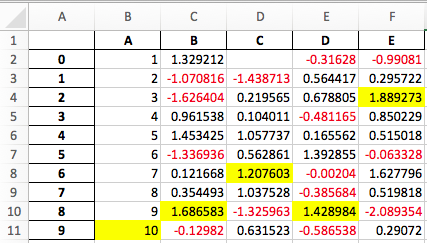
导出到 LaTeX#
(自版本 1.3.0 起)支持将 Styler 导出到 LaTeX。.to_latex 方法的文档提供了更详细的信息和大量示例。
关于 CSS 和 HTML 的更多信息#
层叠样式表(CSS)语言旨在影响浏览器如何渲染 HTML 元素,它有自己的特殊性。它从不报告错误:它只是默默地忽略它们,并且不会按照您的意图渲染您的对象,因此有时可能会令人沮丧。这里简要介绍 Styler 如何创建 HTML 并与 CSS 交互,并提供避免常见陷阱的建议。
CSS 类和 ID#
附加到每个单元格的 CSS class 的精确结构如下。
包含索引和列名称的单元格包括
index_name和level<k>,其中k是其在 MultiIndex 中的级别索引标签单元格包括
行标题level<k>,其中k是 MultiIndex 中的级别row<m>,其中m是行的数字位置
列标签单元格包括
列标题level<k>,其中k是 MultiIndex 中的级别col<n>,其中n是列的数字位置
数据单元格包括
数据row<m>,其中m是单元格的数字位置。col<n>,其中n是单元格的数字位置。
空白单元格包含
blank修剪过的单元格包括
col_trim或row_trim
id 的结构是 T_uuid_level<k>_row<m>_col<n>,其中 level<k> 仅用于标题,并且标题将仅包含 row<m> 或 col<n>,取所需者。默认情况下,我们还在每个行/列标识符前添加了一个对于每个 DataFrame 唯一的 UUID,这样同一个笔记本或页面中的样式就不会与另一个样式冲突。您可以在优化中阅读更多关于 UUID 使用的信息。
我们可以通过调用 .to_html() 方法来查看 HTML 示例。
[71]:
print(pd.DataFrame([[1,2],[3,4]], index=['i1', 'i2'], columns=['c1', 'c2']).style.to_html())
<style type="text/css">
</style>
<table id="T_82d9e">
<thead>
<tr>
<th class="blank level0" > </th>
<th id="T_82d9e_level0_col0" class="col_heading level0 col0" >c1</th>
<th id="T_82d9e_level0_col1" class="col_heading level0 col1" >c2</th>
</tr>
</thead>
<tbody>
<tr>
<th id="T_82d9e_level0_row0" class="row_heading level0 row0" >i1</th>
<td id="T_82d9e_row0_col0" class="data row0 col0" >1</td>
<td id="T_82d9e_row0_col1" class="data row0 col1" >2</td>
</tr>
<tr>
<th id="T_82d9e_level0_row1" class="row_heading level0 row1" >i2</th>
<td id="T_82d9e_row1_col0" class="data row1 col0" >3</td>
<td id="T_82d9e_row1_col1" class="data row1 col1" >4</td>
</tr>
</tbody>
</table>
CSS 层级#
示例表明,当 CSS 样式重叠时,HTML 渲染中最后出现的样式优先。因此,以下代码会产生不同的结果:
[72]:
df4 = pd.DataFrame([['text']])
df4.style.map(lambda x: 'color:green;')\
         .map(lambda x: 'color:red;')
[72]:
| 0 | |
|---|---|
| 0 | 文本 |
[73]:
df4.style.map(lambda x: 'color:red;')\
         .map(lambda x: 'color:green;')
[73]:
| 0 | |
|---|---|
| 0 | 文本 |
这仅适用于层级或重要性相同的 CSS 规则。您可以阅读更多关于CSS 特异性的信息,但为了我们的目的,总结关键点就足够了:
每个 HTML 元素的 CSS 重要性分数通过从零开始并添加以下内容得出:
内联样式属性得 1000 分
每个 ID 得 100 分
每个属性、类或伪类得 10 分
每个元素名称或伪元素得 1 分
我们用这个来描述以下配置的动作
[74]:
df4.style.set_uuid('a_')\
         .set_table_styles([{'selector': 'td', 'props': 'color:red;'}])\
         .map(lambda x: 'color:green;')
[74]:
| 0 | |
|---|---|
| 0 | 文本 |
此文本为红色,因为生成的选择器 #T_a_ td 的值为 101(ID 加元素),而 #T_a_row0_col0 仅为 100(ID),因此即使在 HTML 中它在前面之后,也被认为是次要的。
[75]:
df4.style.set_uuid('b_')\
         .set_table_styles([{'selector': 'td', 'props': 'color:red;'},
                            {'selector': '.cls-1', 'props': 'color:blue;'}])\
         .map(lambda x: 'color:green;')\
         .set_td_classes(pd.DataFrame([['cls-1']]))
[75]:
| 0 | |
|---|---|
| 0 | 文本 |
在上述情况下,文本是蓝色的,因为选择器 #T_b_ .cls-1 的值为 110(ID 加类),它具有优先权。
[76]:
df4.style.set_uuid('c_')\
         .set_table_styles([{'selector': 'td', 'props': 'color:red;'},
                            {'selector': '.cls-1', 'props': 'color:blue;'},
                            {'selector': 'td.data', 'props': 'color:yellow;'}])\
         .map(lambda x: 'color:green;')\
         .set_td_classes(pd.DataFrame([['cls-1']]))
[76]:
| 0 | |
|---|---|
| 0 | 文本 |
现在我们创建了另一个表格样式,这次选择器 T_c_ td.data(ID 加元素加类)的值被提升到 111。
如果您的样式无法应用,并且让您感到非常沮丧,请尝试使用 !important 杀手锏。
[77]:
df4.style.set_uuid('d_')\
         .set_table_styles([{'selector': 'td', 'props': 'color:red;'},
                            {'selector': '.cls-1', 'props': 'color:blue;'},
                            {'selector': 'td.data', 'props': 'color:yellow;'}])\
         .map(lambda x: 'color:green !important;')\
         .set_td_classes(pd.DataFrame([['cls-1']]))
[77]:
| 0 | |
|---|---|
| 0 | 文本 |
终于还是弄出了绿色文本!
可扩展性#
pandas 的核心是并将继续是其“高性能、易于使用的数据结构”。考虑到这一点,我们希望 DataFrame.style 能实现两个目标:
提供一个交互式使用令人愉悦且足以满足许多任务的 API。
为专门的库提供构建基础。
如果您在此基础上构建了一个出色的库,请告知我们,我们将链接到它。
子类化#
如果默认模板不能完全满足您的需求,您可以子类化 Styler 并扩展或覆盖模板。我们将展示一个扩展默认模板以在每个表格前插入自定义标题的示例。
[78]:
from jinja2 import Environment, ChoiceLoader, FileSystemLoader
from IPython.display import HTML
from pandas.io.formats.style import Styler
我们将使用以下模板
[79]:
with open("templates/myhtml.tpl") as f:
    print(f.read())
{% extends "html_table.tpl" %}
{% block table %}
<h1>{{ table_title|default("My Table") }}</h1>
{{ super() }}
{% endblock table %}
现在我们已经创建了一个模板,我们需要设置一个 Styler 的子类,它了解这个模板。Styler
[80]:
class MyStyler(Styler):
    env = Environment(
        loader=ChoiceLoader([
            FileSystemLoader("templates"),  # contains ours
            Styler.loader,  # the default
        ])
    )
    template_html_table = env.get_template("myhtml.tpl")
请注意,我们将原始加载器包含在我们的环境加载器中。这是因为我们扩展了原始模板,所以 Jinja 环境需要能够找到它。
现在我们可以使用那个自定义的 Styler 了。它的 __init__ 接受一个 DataFrame。
[81]:
MyStyler(df3)
[81]:
我的表格
| c1 | c2 | c3 | c4 | ||
|---|---|---|---|---|---|
| A | r1 | -1.048553 | -1.420018 | -1.706270 | 1.950775 |
| r2 | -0.509652 | -0.438074 | -1.252795 | 0.777490 | |
| B | r1 | -1.613898 | -0.212740 | -0.895467 | 0.386902 |
| r2 | -0.510805 | -1.180632 | -0.028182 | 0.428332 |
我们的自定义模板接受一个 table_title 关键字。我们可以在 .to_html 方法中提供该值。
[82]:
HTML(MyStyler(df3).to_html(table_title="Extending Example"))
[82]:
扩展示例
| c1 | c2 | c3 | c4 | ||
|---|---|---|---|---|---|
| A | r1 | -1.048553 | -1.420018 | -1.706270 | 1.950775 |
| r2 | -0.509652 | -0.438074 | -1.252795 | 0.777490 | |
| B | r1 | -1.613898 | -0.212740 | -0.895467 | 0.386902 |
| r2 | -0.510805 | -1.180632 | -0.028182 | 0.428332 |
为方便起见,我们提供了 Styler.from_custom_template 方法,其功能与自定义子类相同。
[83]:
EasyStyler = Styler.from_custom_template("templates", "myhtml.tpl")
HTML(EasyStyler(df3).to_html(table_title="Another Title"))
[83]:
另一个标题
| c1 | c2 | c3 | c4 | ||
|---|---|---|---|---|---|
| A | r1 | -1.048553 | -1.420018 | -1.706270 | 1.950775 |
| r2 | -0.509652 | -0.438074 | -1.252795 | 0.777490 | |
| B | r1 | -1.613898 | -0.212740 | -0.895467 | 0.386902 |
| r2 | -0.510805 | -1.180632 | -0.028182 | 0.428332 |
模板结构#
以下是样式生成模板和表格生成模板的模板结构:
样式模板
[85]:
HTML(style_structure)
[85]:
<style type="text/css">
</style>
表格模板
[87]:
HTML(table_structure)
[87]:
<table ...>
</table>
有关更多详细信息,请参阅 GitHub 仓库中的模板。