索引和选择数据#

pandas 对象中的轴标签信息有多种用途

使用已知指标标识数据（即提供元数据），这对于分析、可视化和交互式控制台显示非常重要。
实现自动和显式数据对齐。
允许直观地获取和设置数据集的子集。

本节我们将重点关注最后一点：即如何对 pandas 对象进行切片、分割，以及一般地获取和设置其子集。主要重点将放在 Series 和 DataFrame 上，因为它们在这方面获得了更多的开发关注。

注意

Python 和 NumPy 的索引运算符 [] 和属性运算符 . 为 pandas 数据结构提供了在各种用例中快速简便的访问方式。这使得交互式操作非常直观，因为如果您已经知道如何处理 Python 字典和 NumPy 数组，那么几乎没有什么新东西需要学习。然而，由于要访问的数据类型无法提前得知，直接使用标准运算符存在一些优化限制。对于生产代码，我们建议您利用本章中介绍的优化后的 pandas 数据访问方法。

警告

设置操作返回的是副本还是引用可能取决于上下文。这有时被称为链式赋值，应尽量避免。参见返回视图而非副本。

有关 MultiIndex 和更高级索引的文档，请参见MultiIndex / 高级索引。

有关一些高级策略，请参见教程。

不同的索引选择#

为了支持更明确的基于位置的索引，对象选择已经增加了一些用户请求的功能。pandas 现在支持三种多轴索引类型。

.loc 主要基于标签，但也可与布尔数组一起使用。当未找到项时，.loc 将引发 KeyError。允许的输入包括
- 单个标签，例如 5 或 'a'（请注意，5 被解释为索引的标签。此用法不是沿索引的整数位置）。
- 标签列表或数组，例如 ['a', 'b', 'c']。
- 带有标签的切片对象，例如 'a':'f'（请注意，与通常的 Python 切片相反，当存在于索引中时，起始和结束都包含在内！参见按标签切片和包含端点。）
- 布尔数组（任何 NA 值都将被视为 False）。
- 一个带有一个参数（调用的 Series 或 DataFrame）并返回有效索引输出（上述之一）的可调用函数。
- 由行（和列）索引组成的元组，其元素是上述输入之一。
更多信息请参见按标签选择。
.iloc 主要基于整数位置（从轴的 0 到 length-1），但也可与布尔数组一起使用。如果请求的索引器超出边界，.iloc 将引发 IndexError，但切片索引器允许超出边界的索引（这符合 Python/NumPy 切片语义）。允许的输入包括
- 整数，例如 5。
- 整数列表或数组，例如 [4, 3, 0]。
- 带有整数的切片对象，例如 1:7。
- 布尔数组（任何 NA 值都将被视为 False）。
- 一个带有一个参数（调用的 Series 或 DataFrame）并返回有效索引输出（上述之一）的可调用函数。
- 由行（和列）索引组成的元组，其元素是上述输入之一。
更多信息请参见按位置选择、高级索引和高级分层索引。
.loc、.iloc 以及 [] 索引都可以接受可调用对象作为索引器。更多信息请参见按可调用对象选择。

注意

在应用可调用对象之前，元组键会解构为行（和列）索引，因此您不能从可调用对象返回元组来同时索引行和列。

使用多轴选择从对象获取值时，使用以下符号（以 .loc 为例，但以下也适用于 .iloc）。任何轴访问器都可以是空切片 :。规范中未包含的轴假定为 :，例如 p.loc['a'] 等同于 p.loc['a', :]。

In [1]: ser = pd.Series(range(5), index=list("abcde"))

In [2]: ser.loc[["a", "c", "e"]]
Out[2]: 
a    0
c    2
e    4
dtype: int64

In [3]: df = pd.DataFrame(np.arange(25).reshape(5, 5), index=list("abcde"), columns=list("abcde"))

In [4]: df.loc[["a", "c", "e"], ["b", "d"]]
Out[4]: 
    b   d
a   1   3
c  11  13
e  21  23

基础知识#

正如在上一节介绍数据结构时提到的，使用 [] 索引（对于熟悉 Python 中实现类行为的人来说，也称为 __getitem__）的主要功能是选择出低维切片。下表显示了使用 [] 索引 pandas 对象时的返回值类型：

对象类型	选择	返回值类型
Series	`series[标签]`	标量值
DataFrame	`frame[列名]`	对应列名的 `Series`

这里我们构建一个简单的时间序列数据集，用于说明索引功能

In [5]: dates = pd.date_range('1/1/2000', periods=8)

In [6]: df = pd.DataFrame(np.random.randn(8, 4),
   ...:                   index=dates, columns=['A', 'B', 'C', 'D'])
   ...: 

In [7]: df
Out[7]: 
                   A         B         C         D
2000-01-01  0.469112 -0.282863 -1.509059 -1.135632
2000-01-02  1.212112 -0.173215  0.119209 -1.044236
2000-01-03 -0.861849 -2.104569 -0.494929  1.071804
2000-01-04  0.721555 -0.706771 -1.039575  0.271860
2000-01-05 -0.424972  0.567020  0.276232 -1.087401
2000-01-06 -0.673690  0.113648 -1.478427  0.524988
2000-01-07  0.404705  0.577046 -1.715002 -1.039268
2000-01-08 -0.370647 -1.157892 -1.344312  0.844885

注意

除非特别说明，否则所有索引功能都不是时间序列特有的。

因此，如上所述，我们使用 [] 进行最基本的索引

In [8]: s = df['A']

In [9]: s[dates[5]]
Out[9]: -0.6736897080883706

您可以将列列表传递给 [] 以按该顺序选择列。如果 DataFrame 中不包含某个列，则会引发异常。也可以通过这种方式设置多个列。

In [10]: df
Out[10]: 
                   A         B         C         D
2000-01-01  0.469112 -0.282863 -1.509059 -1.135632
2000-01-02  1.212112 -0.173215  0.119209 -1.044236
2000-01-03 -0.861849 -2.104569 -0.494929  1.071804
2000-01-04  0.721555 -0.706771 -1.039575  0.271860
2000-01-05 -0.424972  0.567020  0.276232 -1.087401
2000-01-06 -0.673690  0.113648 -1.478427  0.524988
2000-01-07  0.404705  0.577046 -1.715002 -1.039268
2000-01-08 -0.370647 -1.157892 -1.344312  0.844885

In [11]: df[['B', 'A']] = df[['A', 'B']]

In [12]: df
Out[12]: 
                   A         B         C         D
2000-01-01 -0.282863  0.469112 -1.509059 -1.135632
2000-01-02 -0.173215  1.212112  0.119209 -1.044236
2000-01-03 -2.104569 -0.861849 -0.494929  1.071804
2000-01-04 -0.706771  0.721555 -1.039575  0.271860
2000-01-05  0.567020 -0.424972  0.276232 -1.087401
2000-01-06  0.113648 -0.673690 -1.478427  0.524988
2000-01-07  0.577046  0.404705 -1.715002 -1.039268
2000-01-08 -1.157892 -0.370647 -1.344312  0.844885

您可能会发现这对于对列子集应用转换（就地）很有用。

警告

当从 .loc 设置 Series 和 DataFrame 时，pandas 会对齐所有轴。

这**不会**修改 df，因为列对齐发生在值赋值之前。

In [13]: df[['A', 'B']]
Out[13]: 
                   A         B
2000-01-01 -0.282863  0.469112
2000-01-02 -0.173215  1.212112
2000-01-03 -2.104569 -0.861849
2000-01-04 -0.706771  0.721555
2000-01-05  0.567020 -0.424972
2000-01-06  0.113648 -0.673690
2000-01-07  0.577046  0.404705
2000-01-08 -1.157892 -0.370647

In [14]: df.loc[:, ['B', 'A']] = df[['A', 'B']]

In [15]: df[['A', 'B']]
Out[15]: 
                   A         B
2000-01-01 -0.282863  0.469112
2000-01-02 -0.173215  1.212112
2000-01-03 -2.104569 -0.861849
2000-01-04 -0.706771  0.721555
2000-01-05  0.567020 -0.424972
2000-01-06  0.113648 -0.673690
2000-01-07  0.577046  0.404705
2000-01-08 -1.157892 -0.370647

交换列值的正确方法是使用原始值

In [16]: df.loc[:, ['B', 'A']] = df[['A', 'B']].to_numpy()

In [17]: df[['A', 'B']]
Out[17]: 
                   A         B
2000-01-01  0.469112 -0.282863
2000-01-02  1.212112 -0.173215
2000-01-03 -0.861849 -2.104569
2000-01-04  0.721555 -0.706771
2000-01-05 -0.424972  0.567020
2000-01-06 -0.673690  0.113648
2000-01-07  0.404705  0.577046
2000-01-08 -0.370647 -1.157892

然而，当从 .iloc 设置 Series 和 DataFrame 时，pandas 不会对齐轴，因为 .iloc 是按位置操作的。

这将修改 df，因为列对齐没有在值赋值之前完成。

In [18]: df[['A', 'B']]
Out[18]: 
                   A         B
2000-01-01  0.469112 -0.282863
2000-01-02  1.212112 -0.173215
2000-01-03 -0.861849 -2.104569
2000-01-04  0.721555 -0.706771
2000-01-05 -0.424972  0.567020
2000-01-06 -0.673690  0.113648
2000-01-07  0.404705  0.577046
2000-01-08 -0.370647 -1.157892

In [19]: df.iloc[:, [1, 0]] = df[['A', 'B']]

In [20]: df[['A','B']]
Out[20]: 
                   A         B
2000-01-01 -0.282863  0.469112
2000-01-02 -0.173215  1.212112
2000-01-03 -2.104569 -0.861849
2000-01-04 -0.706771  0.721555
2000-01-05  0.567020 -0.424972
2000-01-06  0.113648 -0.673690
2000-01-07  0.577046  0.404705
2000-01-08 -1.157892 -0.370647

属性访问#

您可以直接将 Series 上的索引或 DataFrame 上的列作为属性访问

In [21]: sa = pd.Series([1, 2, 3], index=list('abc'))

In [22]: dfa = df.copy()

In [23]: sa.b
Out[23]: 2

In [24]: dfa.A
Out[24]: 
2000-01-01   -0.282863
2000-01-02   -0.173215
2000-01-03   -2.104569
2000-01-04   -0.706771
2000-01-05    0.567020
2000-01-06    0.113648
2000-01-07    0.577046
2000-01-08   -1.157892
Freq: D, Name: A, dtype: float64

In [25]: sa.a = 5

In [26]: sa
Out[26]: 
a    5
b    2
c    3
dtype: int64

In [27]: dfa.A = list(range(len(dfa.index)))  # ok if A already exists

In [28]: dfa
Out[28]: 
            A         B         C         D
2000-01-01  0  0.469112 -1.509059 -1.135632
2000-01-02  1  1.212112  0.119209 -1.044236
2000-01-03  2 -0.861849 -0.494929  1.071804
2000-01-04  3  0.721555 -1.039575  0.271860
2000-01-05  4 -0.424972  0.276232 -1.087401
2000-01-06  5 -0.673690 -1.478427  0.524988
2000-01-07  6  0.404705 -1.715002 -1.039268
2000-01-08  7 -0.370647 -1.344312  0.844885

In [29]: dfa['A'] = list(range(len(dfa.index)))  # use this form to create a new column

In [30]: dfa
Out[30]: 
            A         B         C         D
2000-01-01  0  0.469112 -1.509059 -1.135632
2000-01-02  1  1.212112  0.119209 -1.044236
2000-01-03  2 -0.861849 -0.494929  1.071804
2000-01-04  3  0.721555 -1.039575  0.271860
2000-01-05  4 -0.424972  0.276232 -1.087401
2000-01-06  5 -0.673690 -1.478427  0.524988
2000-01-07  6  0.404705 -1.715002 -1.039268
2000-01-08  7 -0.370647 -1.344312  0.844885

警告

您只能在索引元素是有效的 Python 标识符时使用此访问方式，例如 s.1 是不允许的。有关有效标识符的解释，请参见此处。
如果属性与现有方法名称冲突，则该属性将不可用，例如 s.min 是不允许的，但 s['min'] 是可以的。
同样，如果属性与以下列表中的任何一个冲突，则该属性将不可用：index、major_axis、minor_axis、items。
在任何这些情况下，标准索引仍然有效，例如 s['1']、s['min'] 和 s['index'] 将访问相应的元素或列。

如果您正在使用 IPython 环境，您还可以使用 Tab 补全来查看这些可访问的属性。

您也可以将 dict 赋值给 DataFrame 的一行。

In [31]: x = pd.DataFrame({'x': [1, 2, 3], 'y': [3, 4, 5]})

In [32]: x.iloc[1] = {'x': 9, 'y': 99}

In [33]: x
Out[33]: 
   x   y
0  1   3
1  9  99
2  3   5

您可以使用属性访问来修改 Series 的现有元素或 DataFrame 的列，但请注意；如果您尝试使用属性访问来创建新列，它会创建一个新属性而不是新列，并因此引发 UserWarning

In [34]: df_new = pd.DataFrame({'one': [1., 2., 3.]})

In [35]: df_new.two = [4, 5, 6]

In [36]: df_new
Out[36]: 
   one
0  1.0
1  2.0
2  3.0

切片范围#

沿任意轴切片范围的最健壮和一致的方法在按位置选择部分中进行了描述，该部分详细介绍了 .iloc 方法。现在，我们解释使用 [] 运算符进行切片的语义。

对于 Series，语法与 ndarray 完全相同，返回值的切片和相应的标签

In [37]: s[:5]
Out[37]: 
2000-01-01    0.469112
2000-01-02    1.212112
2000-01-03   -0.861849
2000-01-04    0.721555
2000-01-05   -0.424972
Freq: D, Name: A, dtype: float64

In [38]: s[::2]
Out[38]: 
2000-01-01    0.469112
2000-01-03   -0.861849
2000-01-05   -0.424972
2000-01-07    0.404705
Freq: 2D, Name: A, dtype: float64

In [39]: s[::-1]
Out[39]: 
2000-01-08   -0.370647
2000-01-07    0.404705
2000-01-06   -0.673690
2000-01-05   -0.424972
2000-01-04    0.721555
2000-01-03   -0.861849
2000-01-02    1.212112
2000-01-01    0.469112
Freq: -1D, Name: A, dtype: float64

请注意，设置也有效。

In [40]: s2 = s.copy()

In [41]: s2[:5] = 0

In [42]: s2
Out[42]: 
2000-01-01    0.000000
2000-01-02    0.000000
2000-01-03    0.000000
2000-01-04    0.000000
2000-01-05    0.000000
2000-01-06   -0.673690
2000-01-07    0.404705
2000-01-08   -0.370647
Freq: D, Name: A, dtype: float64

对于 DataFrame，[] 内部的切片**会切片行**。这主要是作为一种便利提供的，因为它是一种常见的操作。

In [43]: df[:3]
Out[43]: 
                   A         B         C         D
2000-01-01 -0.282863  0.469112 -1.509059 -1.135632
2000-01-02 -0.173215  1.212112  0.119209 -1.044236
2000-01-03 -2.104569 -0.861849 -0.494929  1.071804

In [44]: df[::-1]
Out[44]: 
                   A         B         C         D
2000-01-08 -1.157892 -0.370647 -1.344312  0.844885
2000-01-07  0.577046  0.404705 -1.715002 -1.039268
2000-01-06  0.113648 -0.673690 -1.478427  0.524988
2000-01-05  0.567020 -0.424972  0.276232 -1.087401
2000-01-04 -0.706771  0.721555 -1.039575  0.271860
2000-01-03 -2.104569 -0.861849 -0.494929  1.071804
2000-01-02 -0.173215  1.212112  0.119209 -1.044236
2000-01-01 -0.282863  0.469112 -1.509059 -1.135632

按标签选择#

警告

设置操作返回副本还是引用可能取决于上下文。这有时被称为 链式赋值，应避免。参见返回视图而非副本。

警告

当您提供的切片器与索引类型不兼容（或不可转换）时，.loc 会很严格。例如，在 DatetimeIndex 中使用整数。这将引发 TypeError。

In [45]: dfl = pd.DataFrame(np.random.randn(5, 4),
   ....:                    columns=list('ABCD'),
   ....:                    index=pd.date_range('20130101', periods=5))
   ....: 

In [46]: dfl
Out[46]: 
                   A         B         C         D
2013-01-01  1.075770 -0.109050  1.643563 -1.469388
2013-01-02  0.357021 -0.674600 -1.776904 -0.968914
2013-01-03 -1.294524  0.413738  0.276662 -0.472035
2013-01-04 -0.013960 -0.362543 -0.006154 -0.923061
2013-01-05  0.895717  0.805244 -1.206412  2.565646

In [47]: dfl.loc[2:3]
---------------------------------------------------------------------------
TypeError                                 Traceback (most recent call last)
Cell In[47], line 1
----> 1 dfl.loc[2:3]

File ~/work/pandas/pandas/pandas/core/indexing.py:1191, in _LocationIndexer.__getitem__(self, key)
   1189 maybe_callable = com.apply_if_callable(key, self.obj)
   1190 maybe_callable = self._check_deprecated_callable_usage(key, maybe_callable)
-> 1191 return self._getitem_axis(maybe_callable, axis=axis)

File ~/work/pandas/pandas/pandas/core/indexing.py:1411, in _LocIndexer._getitem_axis(self, key, axis)
   1409 if isinstance(key, slice):
   1410     self._validate_key(key, axis)
-> 1411     return self._get_slice_axis(key, axis=axis)
   1412 elif com.is_bool_indexer(key):
   1413     return self._getbool_axis(key, axis=axis)

File ~/work/pandas/pandas/pandas/core/indexing.py:1443, in _LocIndexer._get_slice_axis(self, slice_obj, axis)
   1440     return obj.copy(deep=False)
   1442 labels = obj._get_axis(axis)
-> 1443 indexer = labels.slice_indexer(slice_obj.start, slice_obj.stop, slice_obj.step)
   1445 if isinstance(indexer, slice):
   1446     return self.obj._slice(indexer, axis=axis)

File ~/work/pandas/pandas/pandas/core/indexes/datetimes.py:682, in DatetimeIndex.slice_indexer(self, start, end, step)
    674 # GH#33146 if start and end are combinations of str and None and Index is not
    675 # monotonic, we can not use Index.slice_indexer because it does not honor the
    676 # actual elements, is only searching for start and end
    677 if (
    678     check_str_or_none(start)
    679     or check_str_or_none(end)
    680     or self.is_monotonic_increasing
    681 ):
--> 682     return Index.slice_indexer(self, start, end, step)
    684 mask = np.array(True)
    685 in_index = True

File ~/work/pandas/pandas/pandas/core/indexes/base.py:6678, in Index.slice_indexer(self, start, end, step)
   6634 def slice_indexer(
   6635     self,
   6636     start: Hashable | None = None,
   6637     end: Hashable | None = None,
   6638     step: int | None = None,
   6639 ) -> slice:
   6640     """
   6641     Compute the slice indexer for input labels and step.
   6642 
   (...)
   6676     slice(1, 3, None)
   6677     """
-> 6678     start_slice, end_slice = self.slice_locs(start, end, step=step)
   6680     # return a slice
   6681     if not is_scalar(start_slice):

File ~/work/pandas/pandas/pandas/core/indexes/base.py:6904, in Index.slice_locs(self, start, end, step)
   6902 start_slice = None
   6903 if start is not None:
-> 6904     start_slice = self.get_slice_bound(start, "left")
   6905 if start_slice is None:
   6906     start_slice = 0

File ~/work/pandas/pandas/pandas/core/indexes/base.py:6819, in Index.get_slice_bound(self, label, side)
   6815 original_label = label
   6817 # For datetime indices label may be a string that has to be converted
   6818 # to datetime boundary according to its resolution.
-> 6819 label = self._maybe_cast_slice_bound(label, side)
   6821 # we need to look up the label
   6822 try:

File ~/work/pandas/pandas/pandas/core/indexes/datetimes.py:642, in DatetimeIndex._maybe_cast_slice_bound(self, label, side)
    637 if isinstance(label, dt.date) and not isinstance(label, dt.datetime):
    638     # Pandas supports slicing with dates, treated as datetimes at midnight.
    639     # https://github.com/pandas-dev/pandas/issues/31501
    640     label = Timestamp(label).to_pydatetime()
--> 642 label = super()._maybe_cast_slice_bound(label, side)
    643 self._data._assert_tzawareness_compat(label)
    644 return Timestamp(label)

File ~/work/pandas/pandas/pandas/core/indexes/datetimelike.py:378, in DatetimeIndexOpsMixin._maybe_cast_slice_bound(self, label, side)
    376     return lower if side == "left" else upper
    377 elif not isinstance(label, self._data._recognized_scalars):
--> 378     self._raise_invalid_indexer("slice", label)
    380 return label

File ~/work/pandas/pandas/pandas/core/indexes/base.py:4308, in Index._raise_invalid_indexer(self, form, key, reraise)
   4306 if reraise is not lib.no_default:
   4307     raise TypeError(msg) from reraise
-> 4308 raise TypeError(msg)

TypeError: cannot do slice indexing on DatetimeIndex with these indexers [2] of type int

切片中的字符串类型可以转换为索引类型，从而实现自然切片。

In [48]: dfl.loc['20130102':'20130104']
Out[48]: 
                   A         B         C         D
2013-01-02  0.357021 -0.674600 -1.776904 -0.968914
2013-01-03 -1.294524  0.413738  0.276662 -0.472035
2013-01-04 -0.013960 -0.362543 -0.006154 -0.923061

pandas 提供了一套方法来实现**纯粹基于标签的索引**。这是一个严格的基于包含的协议。请求的每个标签都必须在索引中，否则将引发 KeyError。切片时，如果起始边界**和**停止边界都在索引中，则它们都将包含在内。整数是有效的标签，但它们指的是标签**而不是位置**。

.loc 属性是主要的访问方法。以下是有效输入

单个标签，例如 5 或 'a'（请注意，5 被解释为索引的标签。此用法不是沿索引的整数位置）。
标签列表或数组，例如 ['a', 'b', 'c']。
带有标签的切片对象，例如 'a':'f'（请注意，与通常的 Python 切片相反，当存在于索引中时，起始和结束**都**包含在内！参见按标签切片。
布尔数组。
一个可调用对象，参见按可调用对象选择。

In [49]: s1 = pd.Series(np.random.randn(6), index=list('abcdef'))

In [50]: s1
Out[50]: 
a    1.431256
b    1.340309
c   -1.170299
d   -0.226169
e    0.410835
f    0.813850
dtype: float64

In [51]: s1.loc['c':]
Out[51]: 
c   -1.170299
d   -0.226169
e    0.410835
f    0.813850
dtype: float64

In [52]: s1.loc['b']
Out[52]: 1.3403088497993827

请注意，设置也有效。

In [53]: s1.loc['c':] = 0

In [54]: s1
Out[54]: 
a    1.431256
b    1.340309
c    0.000000
d    0.000000
e    0.000000
f    0.000000
dtype: float64

对于 DataFrame

In [55]: df1 = pd.DataFrame(np.random.randn(6, 4),
   ....:                    index=list('abcdef'),
   ....:                    columns=list('ABCD'))
   ....: 

In [56]: df1
Out[56]: 
          A         B         C         D
a  0.132003 -0.827317 -0.076467 -1.187678
b  1.130127 -1.436737 -1.413681  1.607920
c  1.024180  0.569605  0.875906 -2.211372
d  0.974466 -2.006747 -0.410001 -0.078638
e  0.545952 -1.219217 -1.226825  0.769804
f -1.281247 -0.727707 -0.121306 -0.097883

In [57]: df1.loc[['a', 'b', 'd'], :]
Out[57]: 
          A         B         C         D
a  0.132003 -0.827317 -0.076467 -1.187678
b  1.130127 -1.436737 -1.413681  1.607920
d  0.974466 -2.006747 -0.410001 -0.078638

通过标签切片访问

In [58]: df1.loc['d':, 'A':'C']
Out[58]: 
          A         B         C
d  0.974466 -2.006747 -0.410001
e  0.545952 -1.219217 -1.226825
f -1.281247 -0.727707 -0.121306

使用标签获取横截面（等同于 df.xs('a')）

In [59]: df1.loc['a']
Out[59]: 
A    0.132003
B   -0.827317
C   -0.076467
D   -1.187678
Name: a, dtype: float64

使用布尔数组获取值

In [60]: df1.loc['a'] > 0
Out[60]: 
A     True
B    False
C    False
D    False
Name: a, dtype: bool

In [61]: df1.loc[:, df1.loc['a'] > 0]
Out[61]: 
          A
a  0.132003
b  1.130127
c  1.024180
d  0.974466
e  0.545952
f -1.281247

布尔数组中的 NA 值传播为 False

In [62]: mask = pd.array([True, False, True, False, pd.NA, False], dtype="boolean")

In [63]: mask
Out[63]: 
<BooleanArray>
[True, False, True, False, <NA>, False]
Length: 6, dtype: boolean

In [64]: df1[mask]
Out[64]: 
          A         B         C         D
a  0.132003 -0.827317 -0.076467 -1.187678
c  1.024180  0.569605  0.875906 -2.211372

显式获取值

# this is also equivalent to ``df1.at['a','A']``
In [65]: df1.loc['a', 'A']
Out[65]: 0.13200317033032932

按标签切片#

当使用 .loc 进行切片时，如果起始标签和停止标签都在索引中，则返回介于两者之间（包括两者）的元素

In [66]: s = pd.Series(list('abcde'), index=[0, 3, 2, 5, 4])

In [67]: s.loc[3:5]
Out[67]: 
3    b
2    c
5    d
dtype: object

如果两者中至少有一个不存在，但索引已排序且可以与起始和停止标签进行比较，则切片仍然会按预期工作，通过选择介于两者之间的排名标签。

In [68]: s.sort_index()
Out[68]: 
0    a
2    c
3    b
4    e
5    d
dtype: object

In [69]: s.sort_index().loc[1:6]
Out[69]: 
2    c
3    b
4    e
5    d
dtype: object

然而，如果两者中至少有一个不存在并且索引未排序，则会引发错误（因为否则计算成本高昂，并且对于混合类型索引可能存在歧义）。例如，在上面的示例中，s.loc[1:6] 将引发 KeyError。

有关此行为的原理，请参见包含端点。

In [70]: s = pd.Series(list('abcdef'), index=[0, 3, 2, 5, 4, 2])

In [71]: s.loc[3:5]
Out[71]: 
3    b
2    c
5    d
dtype: object

此外，如果索引具有重复标签并且起始或停止标签是重复的，则会引发错误。例如，在上面的示例中，s.loc[2:5] 将引发 KeyError。

有关重复标签的更多信息，请参见重复标签。

按位置选择#

警告

设置操作返回副本还是引用可能取决于上下文。这有时被称为 链式赋值，应避免。参见返回视图而非副本。

pandas 提供了一套方法来实现**纯粹基于整数的索引**。其语义与 Python 和 NumPy 的切片非常接近。这是从0开始的索引。切片时，起始边界是包含的，而上限是排除的。尝试使用非整数，即使是**有效**的标签，也将引发 IndexError。

.iloc 属性是主要的访问方法。以下是有效输入

整数，例如 5。
整数列表或数组，例如 [4, 3, 0]。
带有整数的切片对象，例如 1:7。
布尔数组。
一个可调用对象，参见按可调用对象选择。
由行（和列）索引组成的元组，其元素是上述类型之一。

In [72]: s1 = pd.Series(np.random.randn(5), index=list(range(0, 10, 2)))

In [73]: s1
Out[73]: 
0    0.695775
2    0.341734
4    0.959726
6   -1.110336
8   -0.619976
dtype: float64

In [74]: s1.iloc[:3]
Out[74]: 
0    0.695775
2    0.341734
4    0.959726
dtype: float64

In [75]: s1.iloc[3]
Out[75]: -1.110336102891167

请注意，设置也有效。

In [76]: s1.iloc[:3] = 0

In [77]: s1
Out[77]: 
0    0.000000
2    0.000000
4    0.000000
6   -1.110336
8   -0.619976
dtype: float64

对于 DataFrame

In [78]: df1 = pd.DataFrame(np.random.randn(6, 4),
   ....:                    index=list(range(0, 12, 2)),
   ....:                    columns=list(range(0, 8, 2)))
   ....: 

In [79]: df1
Out[79]: 
           0         2         4         6
0   0.149748 -0.732339  0.687738  0.176444
2   0.403310 -0.154951  0.301624 -2.179861
4  -1.369849 -0.954208  1.462696 -1.743161
6  -0.826591 -0.345352  1.314232  0.690579
8   0.995761  2.396780  0.014871  3.357427
10 -0.317441 -1.236269  0.896171 -0.487602

通过整数切片选择

In [80]: df1.iloc[:3]
Out[80]: 
          0         2         4         6
0  0.149748 -0.732339  0.687738  0.176444
2  0.403310 -0.154951  0.301624 -2.179861
4 -1.369849 -0.954208  1.462696 -1.743161

In [81]: df1.iloc[1:5, 2:4]
Out[81]: 
          4         6
2  0.301624 -2.179861
4  1.462696 -1.743161
6  1.314232  0.690579
8  0.014871  3.357427

通过整数列表选择

In [82]: df1.iloc[[1, 3, 5], [1, 3]]
Out[82]: 
           2         6
2  -0.154951 -2.179861
6  -0.345352  0.690579
10 -1.236269 -0.487602

In [83]: df1.iloc[1:3, :]
Out[83]: 
          0         2         4         6
2  0.403310 -0.154951  0.301624 -2.179861
4 -1.369849 -0.954208  1.462696 -1.743161

In [84]: df1.iloc[:, 1:3]
Out[84]: 
           2         4
0  -0.732339  0.687738
2  -0.154951  0.301624
4  -0.954208  1.462696
6  -0.345352  1.314232
8   2.396780  0.014871
10 -1.236269  0.896171

# this is also equivalent to ``df1.iat[1,1]``
In [85]: df1.iloc[1, 1]
Out[85]: -0.1549507744249032

使用整数位置获取横截面（等同于 df.xs(1)）

In [86]: df1.iloc[1]
Out[86]: 
0    0.403310
2   -0.154951
4    0.301624
6   -2.179861
Name: 2, dtype: float64

超出范围的切片索引的处理方式与 Python/NumPy 中一样优雅。

# these are allowed in Python/NumPy.
In [87]: x = list('abcdef')

In [88]: x
Out[88]: ['a', 'b', 'c', 'd', 'e', 'f']

In [89]: x[4:10]
Out[89]: ['e', 'f']

In [90]: x[8:10]
Out[90]: []

In [91]: s = pd.Series(x)

In [92]: s
Out[92]: 
0    a
1    b
2    c
3    d
4    e
5    f
dtype: object

In [93]: s.iloc[4:10]
Out[93]: 
4    e
5    f
dtype: object

In [94]: s.iloc[8:10]
Out[94]: Series([], dtype: object)

请注意，使用超出边界的切片可能会导致空轴（例如，返回一个空的 DataFrame）。

In [95]: dfl = pd.DataFrame(np.random.randn(5, 2), columns=list('AB'))

In [96]: dfl
Out[96]: 
          A         B
0 -0.082240 -2.182937
1  0.380396  0.084844
2  0.432390  1.519970
3 -0.493662  0.600178
4  0.274230  0.132885

In [97]: dfl.iloc[:, 2:3]
Out[97]: 
Empty DataFrame
Columns: []
Index: [0, 1, 2, 3, 4]

In [98]: dfl.iloc[:, 1:3]
Out[98]: 
          B
0 -2.182937
1  0.084844
2  1.519970
3  0.600178
4  0.132885

In [99]: dfl.iloc[4:6]
Out[99]: 
         A         B
4  0.27423  0.132885

单个超出边界的索引器将引发 IndexError。任何元素超出边界的索引器列表将引发 IndexError。

In [100]: dfl.iloc[[4, 5, 6]]
---------------------------------------------------------------------------
IndexError                                Traceback (most recent call last)
File ~/work/pandas/pandas/pandas/core/indexing.py:1714, in _iLocIndexer._get_list_axis(self, key, axis)
   1713 try:
-> 1714     return self.obj._take_with_is_copy(key, axis=axis)
   1715 except IndexError as err:
   1716     # re-raise with different error message, e.g. test_getitem_ndarray_3d

File ~/work/pandas/pandas/pandas/core/generic.py:4172, in NDFrame._take_with_is_copy(self, indices, axis)
   4163 """
   4164 Internal version of the `take` method that sets the `_is_copy`
   4165 attribute to keep track of the parent dataframe (using in indexing
   (...)
   4170 See the docstring of `take` for full explanation of the parameters.
   4171 """
-> 4172 result = self.take(indices=indices, axis=axis)
   4173 # Maybe set copy if we didn't actually change the index.

File ~/work/pandas/pandas/pandas/core/generic.py:4152, in NDFrame.take(self, indices, axis, **kwargs)
   4148     indices = np.arange(
   4149         indices.start, indices.stop, indices.step, dtype=np.intp
   4150     )
-> 4152 new_data = self._mgr.take(
   4153     indices,
   4154     axis=self._get_block_manager_axis(axis),
   4155     verify=True,
   4156 )
   4157 return self._constructor_from_mgr(new_data, axes=new_data.axes).__finalize__(
   4158     self, method="take"
   4159 )

File ~/work/pandas/pandas/pandas/core/internals/managers.py:891, in BaseBlockManager.take(self, indexer, axis, verify)
    890 n = self.shape[axis]
--> 891 indexer = maybe_convert_indices(indexer, n, verify=verify)
    893 new_labels = self.axes[axis].take(indexer)

File ~/work/pandas/pandas/pandas/core/indexers/utils.py:282, in maybe_convert_indices(indices, n, verify)
    281     if mask.any():
--> 282         raise IndexError("indices are out-of-bounds")
    283 return indices

IndexError: indices are out-of-bounds

The above exception was the direct cause of the following exception:

IndexError                                Traceback (most recent call last)
Cell In[100], line 1
----> 1 dfl.iloc[[4, 5, 6]]

File ~/work/pandas/pandas/pandas/core/indexing.py:1191, in _LocationIndexer.__getitem__(self, key)
   1189 maybe_callable = com.apply_if_callable(key, self.obj)
   1190 maybe_callable = self._check_deprecated_callable_usage(key, maybe_callable)
-> 1191 return self._getitem_axis(maybe_callable, axis=axis)

File ~/work/pandas/pandas/pandas/core/indexing.py:1743, in _iLocIndexer._getitem_axis(self, key, axis)
   1741 # a list of integers
   1742 elif is_list_like_indexer(key):
-> 1743     return self._get_list_axis(key, axis=axis)
   1745 # a single integer
   1746 else:
   1747     key = item_from_zerodim(key)

File ~/work/pandas/pandas/pandas/core/indexing.py:1717, in _iLocIndexer._get_list_axis(self, key, axis)
   1714     return self.obj._take_with_is_copy(key, axis=axis)
   1715 except IndexError as err:
   1716     # re-raise with different error message, e.g. test_getitem_ndarray_3d
-> 1717     raise IndexError("positional indexers are out-of-bounds") from err

IndexError: positional indexers are out-of-bounds

In [101]: dfl.iloc[:, 4]
---------------------------------------------------------------------------
IndexError                                Traceback (most recent call last)
Cell In[101], line 1
----> 1 dfl.iloc[:, 4]

File ~/work/pandas/pandas/pandas/core/indexing.py:1184, in _LocationIndexer.__getitem__(self, key)
   1182     if self._is_scalar_access(key):
   1183         return self.obj._get_value(*key, takeable=self._takeable)
-> 1184     return self._getitem_tuple(key)
   1185 else:
   1186     # we by definition only have the 0th axis
   1187     axis = self.axis or 0

File ~/work/pandas/pandas/pandas/core/indexing.py:1690, in _iLocIndexer._getitem_tuple(self, tup)
   1689 def _getitem_tuple(self, tup: tuple):
-> 1690     tup = self._validate_tuple_indexer(tup)
   1691     with suppress(IndexingError):
   1692         return self._getitem_lowerdim(tup)

File ~/work/pandas/pandas/pandas/core/indexing.py:966, in _LocationIndexer._validate_tuple_indexer(self, key)
    964 for i, k in enumerate(key):
    965     try:
--> 966         self._validate_key(k, i)
    967     except ValueError as err:
    968         raise ValueError(
    969             "Location based indexing can only have "
    970             f"[{self._valid_types}] types"
    971         ) from err

File ~/work/pandas/pandas/pandas/core/indexing.py:1592, in _iLocIndexer._validate_key(self, key, axis)
   1590     return
   1591 elif is_integer(key):
-> 1592     self._validate_integer(key, axis)
   1593 elif isinstance(key, tuple):
   1594     # a tuple should already have been caught by this point
   1595     # so don't treat a tuple as a valid indexer
   1596     raise IndexingError("Too many indexers")

File ~/work/pandas/pandas/pandas/core/indexing.py:1685, in _iLocIndexer._validate_integer(self, key, axis)
   1683 len_axis = len(self.obj._get_axis(axis))
   1684 if key >= len_axis or key < -len_axis:
-> 1685     raise IndexError("single positional indexer is out-of-bounds")

IndexError: single positional indexer is out-of-bounds

按可调用对象选择#

.loc、.iloc 以及 [] 索引都可以接受可调用对象作为索引器。该可调用对象必须是一个带有一个参数（调用它的 Series 或 DataFrame）并返回有效索引输出的函数。

注意

对于 .iloc 索引，不支持从可调用对象返回元组，因为行和列索引的元组解构发生在应用可调用对象之前。

In [102]: df1 = pd.DataFrame(np.random.randn(6, 4),
   .....:                    index=list('abcdef'),
   .....:                    columns=list('ABCD'))
   .....: 

In [103]: df1
Out[103]: 
          A         B         C         D
a -0.023688  2.410179  1.450520  0.206053
b -0.251905 -2.213588  1.063327  1.266143
c  0.299368 -0.863838  0.408204 -1.048089
d -0.025747 -0.988387  0.094055  1.262731
e  1.289997  0.082423 -0.055758  0.536580
f -0.489682  0.369374 -0.034571 -2.484478

In [104]: df1.loc[lambda df: df['A'] > 0, :]
Out[104]: 
          A         B         C         D
c  0.299368 -0.863838  0.408204 -1.048089
e  1.289997  0.082423 -0.055758  0.536580

In [105]: df1.loc[:, lambda df: ['A', 'B']]
Out[105]: 
          A         B
a -0.023688  2.410179
b -0.251905 -2.213588
c  0.299368 -0.863838
d -0.025747 -0.988387
e  1.289997  0.082423
f -0.489682  0.369374

In [106]: df1.iloc[:, lambda df: [0, 1]]
Out[106]: 
          A         B
a -0.023688  2.410179
b -0.251905 -2.213588
c  0.299368 -0.863838
d -0.025747 -0.988387
e  1.289997  0.082423
f -0.489682  0.369374

In [107]: df1[lambda df: df.columns[0]]
Out[107]: 
a   -0.023688
b   -0.251905
c    0.299368
d   -0.025747
e    1.289997
f   -0.489682
Name: A, dtype: float64

您可以在 Series 中使用可调用索引。

In [108]: df1['A'].loc[lambda s: s > 0]
Out[108]: 
c    0.299368
e    1.289997
Name: A, dtype: float64

使用这些方法/索引器，您可以链式地进行数据选择操作，而无需使用临时变量。

In [109]: bb = pd.read_csv('data/baseball.csv', index_col='id')

In [110]: (bb.groupby(['year', 'team']).sum(numeric_only=True)
   .....:    .loc[lambda df: df['r'] > 100])
   .....: 
Out[110]: 
           stint    g    ab    r    h  X2b  ...     so   ibb   hbp    sh    sf  gidp
year team                                   ...                                     
2007 CIN       6  379   745  101  203   35  ...  127.0  14.0   1.0   1.0  15.0  18.0
     DET       5  301  1062  162  283   54  ...  176.0   3.0  10.0   4.0   8.0  28.0
     HOU       4  311   926  109  218   47  ...  212.0   3.0   9.0  16.0   6.0  17.0
     LAN      11  413  1021  153  293   61  ...  141.0   8.0   9.0   3.0   8.0  29.0
     NYN      13  622  1854  240  509  101  ...  310.0  24.0  23.0  18.0  15.0  48.0
     SFN       5  482  1305  198  337   67  ...  188.0  51.0   8.0  16.0   6.0  41.0
     TEX       2  198   729  115  200   40  ...  140.0   4.0   5.0   2.0   8.0  16.0
     TOR       4  459  1408  187  378   96  ...  265.0  16.0  12.0   4.0  16.0  38.0

[8 rows x 18 columns]

结合位置和基于标签的索引#

如果您希望从“A”列的索引中获取第 0 个和第 2 个元素，您可以这样做：

In [111]: dfd = pd.DataFrame({'A': [1, 2, 3],
   .....:                     'B': [4, 5, 6]},
   .....:                    index=list('abc'))
   .....: 

In [112]: dfd
Out[112]: 
   A  B
a  1  4
b  2  5
c  3  6

In [113]: dfd.loc[dfd.index[[0, 2]], 'A']
Out[113]: 
a    1
c    3
Name: A, dtype: int64

这也可以使用 .iloc 来表达，通过显式地获取索引器上的位置，并使用位置索引来选择数据。

In [114]: dfd.iloc[[0, 2], dfd.columns.get_loc('A')]
Out[114]: 
a    1
c    3
Name: A, dtype: int64

对于获取多个索引器，使用 .get_indexer

In [115]: dfd.iloc[[0, 2], dfd.columns.get_indexer(['A', 'B'])]
Out[115]: 
   A  B
a  1  4
c  3  6

重新索引#

选择可能不存在的元素的惯用方法是通过 .reindex()。另请参见重新索引部分。

In [116]: s = pd.Series([1, 2, 3])

In [117]: s.reindex([1, 2, 3])
Out[117]: 
1    2.0
2    3.0
3    NaN
dtype: float64

另外，如果您只想选择有效的键，以下方法既惯用又高效；它保证保留选择的数据类型。

In [118]: labels = [1, 2, 3]

In [119]: s.loc[s.index.intersection(labels)]
Out[119]: 
1    2
2    3
dtype: int64

拥有重复索引将为 .reindex() 引发错误。

In [120]: s = pd.Series(np.arange(4), index=['a', 'a', 'b', 'c'])

In [121]: labels = ['c', 'd']

In [122]: s.reindex(labels)
---------------------------------------------------------------------------
ValueError                                Traceback (most recent call last)
Cell In[122], line 1
----> 1 s.reindex(labels)

File ~/work/pandas/pandas/pandas/core/series.py:5164, in Series.reindex(self, index, axis, method, copy, level, fill_value, limit, tolerance)
   5147 @doc(
   5148     NDFrame.reindex,  # type: ignore[has-type]
   5149     klass=_shared_doc_kwargs["klass"],
   (...)
   5162     tolerance=None,
   5163 ) -> Series:
-> 5164     return super().reindex(
   5165         index=index,
   5166         method=method,
   5167         copy=copy,
   5168         level=level,
   5169         fill_value=fill_value,
   5170         limit=limit,
   5171         tolerance=tolerance,
   5172     )

File ~/work/pandas/pandas/pandas/core/generic.py:5629, in NDFrame.reindex(self, labels, index, columns, axis, method, copy, level, fill_value, limit, tolerance)
   5626     return self._reindex_multi(axes, copy, fill_value)
   5628 # perform the reindex on the axes
-> 5629 return self._reindex_axes(
   5630     axes, level, limit, tolerance, method, fill_value, copy
   5631 ).__finalize__(self, method="reindex")

File ~/work/pandas/pandas/pandas/core/generic.py:5652, in NDFrame._reindex_axes(self, axes, level, limit, tolerance, method, fill_value, copy)
   5649     continue
   5651 ax = self._get_axis(a)
-> 5652 new_index, indexer = ax.reindex(
   5653     labels, level=level, limit=limit, tolerance=tolerance, method=method
   5654 )
   5656 axis = self._get_axis_number(a)
   5657 obj = obj._reindex_with_indexers(
   5658     {axis: [new_index, indexer]},
   5659     fill_value=fill_value,
   5660     copy=copy,
   5661     allow_dups=False,
   5662 )

File ~/work/pandas/pandas/pandas/core/indexes/base.py:4436, in Index.reindex(self, target, method, level, limit, tolerance)
   4433     raise ValueError("cannot handle a non-unique multi-index!")
   4434 elif not self.is_unique:
   4435     # GH#42568
-> 4436     raise ValueError("cannot reindex on an axis with duplicate labels")
   4437 else:
   4438     indexer, _ = self.get_indexer_non_unique(target)

ValueError: cannot reindex on an axis with duplicate labels

通常，您可以将所需的标签与当前轴求交集，然后重新索引。

In [123]: s.loc[s.index.intersection(labels)].reindex(labels)
Out[123]: 
c    3.0
d    NaN
dtype: float64

然而，如果您的结果索引是重复的，这仍然会引发错误。

In [124]: labels = ['a', 'd']

In [125]: s.loc[s.index.intersection(labels)].reindex(labels)
---------------------------------------------------------------------------
ValueError                                Traceback (most recent call last)
Cell In[125], line 1
----> 1 s.loc[s.index.intersection(labels)].reindex(labels)

File ~/work/pandas/pandas/pandas/core/series.py:5164, in Series.reindex(self, index, axis, method, copy, level, fill_value, limit, tolerance)
   5147 @doc(
   5148     NDFrame.reindex,  # type: ignore[has-type]
   5149     klass=_shared_doc_kwargs["klass"],
   (...)
   5162     tolerance=None,
   5163 ) -> Series:
-> 5164     return super().reindex(
   5165         index=index,
   5166         method=method,
   5167         copy=copy,
   5168         level=level,
   5169         fill_value=fill_value,
   5170         limit=limit,
   5171         tolerance=tolerance,
   5172     )

File ~/work/pandas/pandas/pandas/core/generic.py:5629, in NDFrame.reindex(self, labels, index, columns, axis, method, copy, level, fill_value, limit, tolerance)
   5626     return self._reindex_multi(axes, copy, fill_value)
   5628 # perform the reindex on the axes
-> 5629 return self._reindex_axes(
   5630     axes, level, limit, tolerance, method, fill_value, copy
   5631 ).__finalize__(self, method="reindex")

File ~/work/pandas/pandas/pandas/core/generic.py:5652, in NDFrame._reindex_axes(self, axes, level, limit, tolerance, method, fill_value, copy)
   5649     continue
   5651 ax = self._get_axis(a)
-> 5652 new_index, indexer = ax.reindex(
   5653     labels, level=level, limit=limit, tolerance=tolerance, method=method
   5654 )
   5656 axis = self._get_axis_number(a)
   5657 obj = obj._reindex_with_indexers(
   5658     {axis: [new_index, indexer]},
   5659     fill_value=fill_value,
   5660     copy=copy,
   5661     allow_dups=False,
   5662 )

File ~/work/pandas/pandas/pandas/core/indexes/base.py:4436, in Index.reindex(self, target, method, level, limit, tolerance)
   4433     raise ValueError("cannot handle a non-unique multi-index!")
   4434 elif not self.is_unique:
   4435     # GH#42568
-> 4436     raise ValueError("cannot reindex on an axis with duplicate labels")
   4437 else:
   4438     indexer, _ = self.get_indexer_non_unique(target)

ValueError: cannot reindex on an axis with duplicate labels

选择随机样本#

使用 sample() 方法从 Series 或 DataFrame 中随机选择行或列。该方法默认会采样行，并接受指定数量的行/列或行的一部分。

In [126]: s = pd.Series([0, 1, 2, 3, 4, 5])

# When no arguments are passed, returns 1 row.
In [127]: s.sample()
Out[127]: 
4    4
dtype: int64

# One may specify either a number of rows:
In [128]: s.sample(n=3)
Out[128]: 
0    0
4    4
1    1
dtype: int64

# Or a fraction of the rows:
In [129]: s.sample(frac=0.5)
Out[129]: 
5    5
3    3
1    1
dtype: int64

默认情况下，sample 将最多返回每行一次，但也可以使用 replace 选项进行有放回抽样。

In [130]: s = pd.Series([0, 1, 2, 3, 4, 5])

# Without replacement (default):
In [131]: s.sample(n=6, replace=False)
Out[131]: 
0    0
1    1
5    5
3    3
2    2
4    4
dtype: int64

# With replacement:
In [132]: s.sample(n=6, replace=True)
Out[132]: 
0    0
4    4
3    3
2    2
4    4
4    4
dtype: int64

默认情况下，每行被选中的概率相等，但如果您希望行具有不同的概率，您可以将抽样权重作为 weights 传递给 sample 函数。这些权重可以是列表、NumPy 数组或 Series，但它们必须与您抽样对象的长度相同。缺失值将被视为权重为零，不允许使用 inf 值。如果权重之和不为 1，它们将通过将所有权重除以权重之和进行重新归一化。例如

In [133]: s = pd.Series([0, 1, 2, 3, 4, 5])

In [134]: example_weights = [0, 0, 0.2, 0.2, 0.2, 0.4]

In [135]: s.sample(n=3, weights=example_weights)
Out[135]: 
5    5
4    4
3    3
dtype: int64

# Weights will be re-normalized automatically
In [136]: example_weights2 = [0.5, 0, 0, 0, 0, 0]

In [137]: s.sample(n=1, weights=example_weights2)
Out[137]: 
0    0
dtype: int64

当应用于 DataFrame 时，您可以通过简单地将列名作为字符串传递，从而使用 DataFrame 的列作为抽样权重（前提是您正在抽样行而非列）。

In [138]: df2 = pd.DataFrame({'col1': [9, 8, 7, 6],
   .....:                     'weight_column': [0.5, 0.4, 0.1, 0]})
   .....: 

In [139]: df2.sample(n=3, weights='weight_column')
Out[139]: 
   col1  weight_column
1     8            0.4
0     9            0.5
2     7            0.1

sample 也允许用户使用 axis 参数抽取列而不是行。

In [140]: df3 = pd.DataFrame({'col1': [1, 2, 3], 'col2': [2, 3, 4]})

In [141]: df3.sample(n=1, axis=1)
Out[141]: 
   col1
0     1
1     2
2     3

最后，还可以使用 random_state 参数为 sample 的随机数生成器设置种子，该参数将接受整数（作为种子）或 NumPy RandomState 对象。

In [142]: df4 = pd.DataFrame({'col1': [1, 2, 3], 'col2': [2, 3, 4]})

# With a given seed, the sample will always draw the same rows.
In [143]: df4.sample(n=2, random_state=2)
Out[143]: 
   col1  col2
2     3     4
1     2     3

In [144]: df4.sample(n=2, random_state=2)
Out[144]: 
   col1  col2
2     3     4
1     2     3

伴随扩展的设置#

当为某个轴设置不存在的键时，.loc/[] 操作可以执行扩展。

在 Series 的情况下，这实际上是一个追加操作。

In [145]: se = pd.Series([1, 2, 3])

In [146]: se
Out[146]: 
0    1
1    2
2    3
dtype: int64

In [147]: se[5] = 5.

In [148]: se
Out[148]: 
0    1.0
1    2.0
2    3.0
5    5.0
dtype: float64

DataFrame 可以通过 .loc 在任一轴上进行扩展。

In [149]: dfi = pd.DataFrame(np.arange(6).reshape(3, 2),
   .....:                    columns=['A', 'B'])
   .....: 

In [150]: dfi
Out[150]: 
   A  B
0  0  1
1  2  3
2  4  5

In [151]: dfi.loc[:, 'C'] = dfi.loc[:, 'A']

In [152]: dfi
Out[152]: 
   A  B  C
0  0  1  0
1  2  3  2
2  4  5  4

这就像在 DataFrame 上执行 append 操作。

In [153]: dfi.loc[3] = 5

In [154]: dfi
Out[154]: 
   A  B  C
0  0  1  0
1  2  3  2
2  4  5  4
3  5  5  5

快速获取和设置标量值#

由于使用 [] 进行索引必须处理许多情况（单标签访问、切片、布尔索引等），因此它在确定您的请求时会产生一些开销。如果您只想访问标量值，最快的方法是使用 at 和 iat 方法，这些方法在所有数据结构上都已实现。

类似于 loc，at 提供**基于标签**的标量查找，而 iat 类似 iloc 提供**基于整数**的查找。

In [155]: s.iat[5]
Out[155]: 5

In [156]: df.at[dates[5], 'A']
Out[156]: 0.1136484096888855

In [157]: df.iat[3, 0]
Out[157]: -0.7067711336300845

您也可以使用这些相同的索引器进行设置。

In [158]: df.at[dates[5], 'E'] = 7

In [159]: df.iat[3, 0] = 7

如果索引器缺失，at 可能会像上面那样就地扩展对象。

In [160]: df.at[dates[-1] + pd.Timedelta('1 day'), 0] = 7

In [161]: df
Out[161]: 
                   A         B         C         D    E    0
2000-01-01 -0.282863  0.469112 -1.509059 -1.135632  NaN  NaN
2000-01-02 -0.173215  1.212112  0.119209 -1.044236  NaN  NaN
2000-01-03 -2.104569 -0.861849 -0.494929  1.071804  NaN  NaN
2000-01-04  7.000000  0.721555 -1.039575  0.271860  NaN  NaN
2000-01-05  0.567020 -0.424972  0.276232 -1.087401  NaN  NaN
2000-01-06  0.113648 -0.673690 -1.478427  0.524988  7.0  NaN
2000-01-07  0.577046  0.404705 -1.715002 -1.039268  NaN  NaN
2000-01-08 -1.157892 -0.370647 -1.344312  0.844885  NaN  NaN
2000-01-09       NaN       NaN       NaN       NaN  NaN  7.0

布尔索引#

另一种常见的操作是使用布尔向量来筛选数据。运算符包括：| 表示 or，& 表示 and，~ 表示 not。这些操作**必须**使用括号进行分组，因为默认情况下 Python 会将 df['A'] > 2 & df['B'] < 3 这样的表达式评估为 df['A'] > (2 & df['B']) < 3，而期望的评估顺序是 (df['A'] > 2) & (df['B'] < 3)。

使用布尔向量索引 Series 的方式与 NumPy ndarray 中完全相同。

In [162]: s = pd.Series(range(-3, 4))

In [163]: s
Out[163]: 
0   -3
1   -2
2   -1
3    0
4    1
5    2
6    3
dtype: int64

In [164]: s[s > 0]
Out[164]: 
4    1
5    2
6    3
dtype: int64

In [165]: s[(s < -1) | (s > 0.5)]
Out[165]: 
0   -3
1   -2
4    1
5    2
6    3
dtype: int64

In [166]: s[~(s < 0)]
Out[166]: 
3    0
4    1
5    2
6    3
dtype: int64

您可以使用与 DataFrame 索引长度相同的布尔向量（例如，从 DataFrame 的某列派生出的布尔向量）来选择 DataFrame 中的行。

In [167]: df[df['A'] > 0]
Out[167]: 
                   A         B         C         D    E   0
2000-01-04  7.000000  0.721555 -1.039575  0.271860  NaN NaN
2000-01-05  0.567020 -0.424972  0.276232 -1.087401  NaN NaN
2000-01-06  0.113648 -0.673690 -1.478427  0.524988  7.0 NaN
2000-01-07  0.577046  0.404705 -1.715002 -1.039268  NaN NaN

列表推导式和 Series 的 map 方法也可以用于生成更复杂的条件。

In [168]: df2 = pd.DataFrame({'a': ['one', 'one', 'two', 'three', 'two', 'one', 'six'],
   .....:                     'b': ['x', 'y', 'y', 'x', 'y', 'x', 'x'],
   .....:                     'c': np.random.randn(7)})
   .....: 

# only want 'two' or 'three'
In [169]: criterion = df2['a'].map(lambda x: x.startswith('t'))

In [170]: df2[criterion]
Out[170]: 
       a  b         c
2    two  y  0.041290
3  three  x  0.361719
4    two  y -0.238075

# equivalent but slower
In [171]: df2[[x.startswith('t') for x in df2['a']]]
Out[171]: 
       a  b         c
2    two  y  0.041290
3  three  x  0.361719
4    two  y -0.238075

# Multiple criteria
In [172]: df2[criterion & (df2['b'] == 'x')]
Out[172]: 
       a  b         c
3  three  x  0.361719

结合按标签选择、按位置选择和高级索引这些方法，您可以使用布尔向量与其他索引表达式结合，沿多个轴进行选择。

In [173]: df2.loc[criterion & (df2['b'] == 'x'), 'b':'c']
Out[173]: 
   b         c
3  x  0.361719

警告

iloc 支持两种布尔索引。如果索引器是布尔 Series，则会引发错误。例如，在下面的示例中，df.iloc[s.values, 1] 是可以的。布尔索引器是一个数组。但是 df.iloc[s, 1] 会引发 ValueError。

In [174]: df = pd.DataFrame([[1, 2], [3, 4], [5, 6]],
   .....:                   index=list('abc'),
   .....:                   columns=['A', 'B'])
   .....: 

In [175]: s = (df['A'] > 2)

In [176]: s
Out[176]: 
a    False
b     True
c     True
Name: A, dtype: bool

In [177]: df.loc[s, 'B']
Out[177]: 
b    4
c    6
Name: B, dtype: int64

In [178]: df.iloc[s.values, 1]
Out[178]: 
b    4
c    6
Name: B, dtype: int64

使用 isin 进行索引#

考虑 Series 的 isin() 方法，它返回一个布尔向量，当 Series 元素存在于传递的列表中时，该向量为 True。这允许您选择一个或多个列包含您所需值的行。

In [179]: s = pd.Series(np.arange(5), index=np.arange(5)[::-1], dtype='int64')

In [180]: s
Out[180]: 
4    0
3    1
2    2
1    3
0    4
dtype: int64

In [181]: s.isin([2, 4, 6])
Out[181]: 
4    False
3    False
2     True
1    False
0     True
dtype: bool

In [182]: s[s.isin([2, 4, 6])]
Out[182]: 
2    2
0    4
dtype: int64

相同的方法也可用于 Index 对象，在您不确定所查找的哪些标签实际存在时很有用。

In [183]: s[s.index.isin([2, 4, 6])]
Out[183]: 
4    0
2    2
dtype: int64

# compare it to the following
In [184]: s.reindex([2, 4, 6])
Out[184]: 
2    2.0
4    0.0
6    NaN
dtype: float64

此外，MultiIndex 允许选择一个单独的级别用于成员资格检查。

In [185]: s_mi = pd.Series(np.arange(6),
   .....:                  index=pd.MultiIndex.from_product([[0, 1], ['a', 'b', 'c']]))
   .....: 

In [186]: s_mi
Out[186]: 
0  a    0
   b    1
   c    2
1  a    3
   b    4
   c    5
dtype: int64

In [187]: s_mi.iloc[s_mi.index.isin([(1, 'a'), (2, 'b'), (0, 'c')])]
Out[187]: 
0  c    2
1  a    3
dtype: int64

In [188]: s_mi.iloc[s_mi.index.isin(['a', 'c', 'e'], level=1)]
Out[188]: 
0  a    0
   c    2
1  a    3
   c    5
dtype: int64

DataFrame 也有一个 isin() 方法。调用 isin 时，将一组值作为数组或字典传递。如果 values 是一个数组，isin 返回一个与原始 DataFrame 形状相同的布尔 DataFrame，其中元素在值序列中时为 True。

In [189]: df = pd.DataFrame({'vals': [1, 2, 3, 4], 'ids': ['a', 'b', 'f', 'n'],
   .....:                    'ids2': ['a', 'n', 'c', 'n']})
   .....: 

In [190]: values = ['a', 'b', 1, 3]

In [191]: df.isin(values)
Out[191]: 
    vals    ids   ids2
0   True   True   True
1  False   True  False
2   True  False  False
3  False  False  False

通常您会希望将某些值与某些列进行匹配。只需将 values 设置为 dict，其中键是列名，值是您要检查的项目列表即可。

In [192]: values = {'ids': ['a', 'b'], 'vals': [1, 3]}

In [193]: df.isin(values)
Out[193]: 
    vals    ids   ids2
0   True   True  False
1  False   True  False
2   True  False  False
3  False  False  False

要返回一个布尔型 DataFrame，其中值不在原始 DataFrame 中，请使用 ~ 运算符。

In [194]: values = {'ids': ['a', 'b'], 'vals': [1, 3]}

In [195]: ~df.isin(values)
Out[195]: 
    vals    ids  ids2
0  False  False  True
1   True  False  True
2  False   True  True
3   True   True  True

将 DataFrame 的 isin 与 any() 和 all() 方法结合使用，可以快速选择满足给定条件的数据子集。要选择每一列都满足自身条件的行：

In [196]: values = {'ids': ['a', 'b'], 'ids2': ['a', 'c'], 'vals': [1, 3]}

In [197]: row_mask = df.isin(values).all(1)

In [198]: df[row_mask]
Out[198]: 
   vals ids ids2
0     1   a    a

`where()` 方法和掩码#

使用布尔向量从 Series 中选择值通常会返回数据的一个子集。为了保证选择输出与原始数据具有相同的形状，您可以使用 Series 和 DataFrame 中的 where 方法。

只返回选定的行

In [199]: s[s > 0]
Out[199]: 
3    1
2    2
1    3
0    4
dtype: int64

返回与原始 Series 相同形状的 Series

In [200]: s.where(s > 0)
Out[200]: 
4    NaN
3    1.0
2    2.0
1    3.0
0    4.0
dtype: float64

现在，使用布尔条件从 DataFrame 中选择值也能保留输入数据的形状。where 在底层用作实现。以下代码等同于 df.where(df < 0)。

In [201]: dates = pd.date_range('1/1/2000', periods=8)

In [202]: df = pd.DataFrame(np.random.randn(8, 4),
   .....:                   index=dates, columns=['A', 'B', 'C', 'D'])
   .....: 

In [203]: df[df < 0]
Out[203]: 
                   A         B         C         D
2000-01-01 -2.104139 -1.309525       NaN       NaN
2000-01-02 -0.352480       NaN -1.192319       NaN
2000-01-03 -0.864883       NaN -0.227870       NaN
2000-01-04       NaN -1.222082       NaN -1.233203
2000-01-05       NaN -0.605656 -1.169184       NaN
2000-01-06       NaN -0.948458       NaN -0.684718
2000-01-07 -2.670153 -0.114722       NaN -0.048048
2000-01-08       NaN       NaN -0.048788 -0.808838

此外，where 接受一个可选的 other 参数，用于在返回的副本中替换条件为 False 的值。

In [204]: df.where(df < 0, -df)
Out[204]: 
                   A         B         C         D
2000-01-01 -2.104139 -1.309525 -0.485855 -0.245166
2000-01-02 -0.352480 -0.390389 -1.192319 -1.655824
2000-01-03 -0.864883 -0.299674 -0.227870 -0.281059
2000-01-04 -0.846958 -1.222082 -0.600705 -1.233203
2000-01-05 -0.669692 -0.605656 -1.169184 -0.342416
2000-01-06 -0.868584 -0.948458 -2.297780 -0.684718
2000-01-07 -2.670153 -0.114722 -0.168904 -0.048048
2000-01-08 -0.801196 -1.392071 -0.048788 -0.808838

您可能希望根据某些布尔条件设置值。这可以直观地完成，如下所示：

In [205]: s2 = s.copy()

In [206]: s2[s2 < 0] = 0

In [207]: s2
Out[207]: 
4    0
3    1
2    2
1    3
0    4
dtype: int64

In [208]: df2 = df.copy()

In [209]: df2[df2 < 0] = 0

In [210]: df2
Out[210]: 
                   A         B         C         D
2000-01-01  0.000000  0.000000  0.485855  0.245166
2000-01-02  0.000000  0.390389  0.000000  1.655824
2000-01-03  0.000000  0.299674  0.000000  0.281059
2000-01-04  0.846958  0.000000  0.600705  0.000000
2000-01-05  0.669692  0.000000  0.000000  0.342416
2000-01-06  0.868584  0.000000  2.297780  0.000000
2000-01-07  0.000000  0.000000  0.168904  0.000000
2000-01-08  0.801196  1.392071  0.000000  0.000000

where 返回数据的修改副本。

注意

DataFrame.where() 的签名与 numpy.where() 不同。大致上，df1.where(m, df2) 等同于 np.where(m, df1, df2)。

In [211]: df.where(df < 0, -df) == np.where(df < 0, df, -df)
Out[211]: 
               A     B     C     D
2000-01-01  True  True  True  True
2000-01-02  True  True  True  True
2000-01-03  True  True  True  True
2000-01-04  True  True  True  True
2000-01-05  True  True  True  True
2000-01-06  True  True  True  True
2000-01-07  True  True  True  True
2000-01-08  True  True  True  True

对齐

此外，where 会对齐输入的布尔条件（ndarray 或 DataFrame），从而实现带有设置的部分选择。这类似于通过 .loc 进行部分设置（但作用于内容而非轴标签）。

In [212]: df2 = df.copy()

In [213]: df2[df2[1:4] > 0] = 3

In [214]: df2
Out[214]: 
                   A         B         C         D
2000-01-01 -2.104139 -1.309525  0.485855  0.245166
2000-01-02 -0.352480  3.000000 -1.192319  3.000000
2000-01-03 -0.864883  3.000000 -0.227870  3.000000
2000-01-04  3.000000 -1.222082  3.000000 -1.233203
2000-01-05  0.669692 -0.605656 -1.169184  0.342416
2000-01-06  0.868584 -0.948458  2.297780 -0.684718
2000-01-07 -2.670153 -0.114722  0.168904 -0.048048
2000-01-08  0.801196  1.392071 -0.048788 -0.808838

`where` 还可以接受 axis 和 level 参数，以便在执行 where 时对齐输入。

In [215]: df2 = df.copy()

In [216]: df2.where(df2 > 0, df2['A'], axis='index')
Out[216]: 
                   A         B         C         D
2000-01-01 -2.104139 -2.104139  0.485855  0.245166
2000-01-02 -0.352480  0.390389 -0.352480  1.655824
2000-01-03 -0.864883  0.299674 -0.864883  0.281059
2000-01-04  0.846958  0.846958  0.600705  0.846958
2000-01-05  0.669692  0.669692  0.669692  0.342416
2000-01-06  0.868584  0.868584  2.297780  0.868584
2000-01-07 -2.670153 -2.670153  0.168904 -2.670153
2000-01-08  0.801196  1.392071  0.801196  0.801196

这等同于（但快于）以下操作。

In [217]: df2 = df.copy()

In [218]: df.apply(lambda x, y: x.where(x > 0, y), y=df['A'])
Out[218]: 
                   A         B         C         D
2000-01-01 -2.104139 -2.104139  0.485855  0.245166
2000-01-02 -0.352480  0.390389 -0.352480  1.655824
2000-01-03 -0.864883  0.299674 -0.864883  0.281059
2000-01-04  0.846958  0.846958  0.600705  0.846958
2000-01-05  0.669692  0.669692  0.669692  0.342416
2000-01-06  0.868584  0.868584  2.297780  0.868584
2000-01-07 -2.670153 -2.670153  0.168904 -2.670153
2000-01-08  0.801196  1.392071  0.801196  0.801196

where 可以接受可调用对象作为条件和 other 参数。该函数必须带有一个参数（调用的 Series 或 DataFrame），并返回有效的输出作为条件和 other 参数。

In [219]: df3 = pd.DataFrame({'A': [1, 2, 3],
   .....:                     'B': [4, 5, 6],
   .....:                     'C': [7, 8, 9]})
   .....: 

In [220]: df3.where(lambda x: x > 4, lambda x: x + 10)
Out[220]: 
    A   B  C
0  11  14  7
1  12   5  8
2  13   6  9

掩码#

mask() 是 where 的反向布尔操作。

In [221]: s.mask(s >= 0)
Out[221]: 
4   NaN
3   NaN
2   NaN
1   NaN
0   NaN
dtype: float64

In [222]: df.mask(df >= 0)
Out[222]: 
                   A         B         C         D
2000-01-01 -2.104139 -1.309525       NaN       NaN
2000-01-02 -0.352480       NaN -1.192319       NaN
2000-01-03 -0.864883       NaN -0.227870       NaN
2000-01-04       NaN -1.222082       NaN -1.233203
2000-01-05       NaN -0.605656 -1.169184       NaN
2000-01-06       NaN -0.948458       NaN -0.684718
2000-01-07 -2.670153 -0.114722       NaN -0.048048
2000-01-08       NaN       NaN -0.048788 -0.808838

使用 `numpy()` 有条件地进行扩展设置#

where() 的一个替代方法是使用 numpy.where()。结合设置新列，您可以使用它来扩展 DataFrame，其中值是根据条件确定的。

假设您在以下 DataFrame 中有两个选择。当第二列包含“Z”时，您想将新列的颜色设置为“绿色”。您可以这样做：

In [223]: df = pd.DataFrame({'col1': list('ABBC'), 'col2': list('ZZXY')})

In [224]: df['color'] = np.where(df['col2'] == 'Z', 'green', 'red')

In [225]: df
Out[225]: 
  col1 col2  color
0    A    Z  green
1    B    Z  green
2    B    X    red
3    C    Y    red

如果您有多个条件，可以使用 numpy.select() 来实现。例如，对应于三个条件有三种颜色选择，并有一个第四种颜色作为备选，您可以这样做：

In [226]: conditions = [
   .....:     (df['col2'] == 'Z') & (df['col1'] == 'A'),
   .....:     (df['col2'] == 'Z') & (df['col1'] == 'B'),
   .....:     (df['col1'] == 'B')
   .....: ]
   .....: 

In [227]: choices = ['yellow', 'blue', 'purple']

In [228]: df['color'] = np.select(conditions, choices, default='black')

In [229]: df
Out[229]: 
  col1 col2   color
0    A    Z  yellow
1    B    Z    blue
2    B    X  purple
3    C    Y   black

`query()` 方法#

DataFrame 对象有一个 query() 方法，允许使用表达式进行选择。

您可以获取框架中列 b 的值介于列 a 和 c 的值之间的部分。例如

In [230]: n = 10

In [231]: df = pd.DataFrame(np.random.rand(n, 3), columns=list('abc'))

In [232]: df
Out[232]: 
          a         b         c
0  0.438921  0.118680  0.863670
1  0.138138  0.577363  0.686602
2  0.595307  0.564592  0.520630
3  0.913052  0.926075  0.616184
4  0.078718  0.854477  0.898725
5  0.076404  0.523211  0.591538
6  0.792342  0.216974  0.564056
7  0.397890  0.454131  0.915716
8  0.074315  0.437913  0.019794
9  0.559209  0.502065  0.026437

# pure python
In [233]: df[(df['a'] < df['b']) & (df['b'] < df['c'])]
Out[233]: 
          a         b         c
1  0.138138  0.577363  0.686602
4  0.078718  0.854477  0.898725
5  0.076404  0.523211  0.591538
7  0.397890  0.454131  0.915716

# query
In [234]: df.query('(a < b) & (b < c)')
Out[234]: 
          a         b         c
1  0.138138  0.577363  0.686602
4  0.078718  0.854477  0.898725
5  0.076404  0.523211  0.591538
7  0.397890  0.454131  0.915716

执行相同的操作，但如果没有名为 a 的列，则回退到命名索引。

In [235]: df = pd.DataFrame(np.random.randint(n / 2, size=(n, 2)), columns=list('bc'))

In [236]: df.index.name = 'a'

In [237]: df
Out[237]: 
   b  c
a      
0  0  4
1  0  1
2  3  4
3  4  3
4  1  4
5  0  3
6  0  1
7  3  4
8  2  3
9  1  1

In [238]: df.query('a < b and b < c')
Out[238]: 
   b  c
a      
2  3  4

如果您不想或无法命名索引，可以在查询表达式中使用名称 index。

In [239]: df = pd.DataFrame(np.random.randint(n, size=(n, 2)), columns=list('bc'))

In [240]: df
Out[240]: 
   b  c
0  3  1
1  3  0
2  5  6
3  5  2
4  7  4
5  0  1
6  2  5
7  0  1
8  6  0
9  7  9

In [241]: df.query('index < b < c')
Out[241]: 
   b  c
2  5  6

注意

如果索引的名称与列名重叠，则列名具有优先权。例如，

In [242]: df = pd.DataFrame({'a': np.random.randint(5, size=5)})

In [243]: df.index.name = 'a'

In [244]: df.query('a > 2')  # uses the column 'a', not the index
Out[244]: 
   a
a   
1  3
3  3

您仍然可以使用特殊标识符“index”在查询表达式中使用索引。

In [245]: df.query('index > 2')
Out[245]: 
   a
a   
3  3
4  2

如果由于某种原因您有一个名为 index 的列，那么您也可以将索引称为 ilevel_0，但此时您应该考虑将列重命名为不那么模棱两可的名称。

`MultiIndex` `query()` 语法#

您也可以将带有 MultiIndex 的 DataFrame 的级别用作框架中的列。

In [246]: n = 10

In [247]: colors = np.random.choice(['red', 'green'], size=n)

In [248]: foods = np.random.choice(['eggs', 'ham'], size=n)

In [249]: colors
Out[249]: 
array(['red', 'red', 'red', 'green', 'green', 'green', 'green', 'green',
       'green', 'green'], dtype='<U5')

In [250]: foods
Out[250]: 
array(['ham', 'ham', 'eggs', 'eggs', 'eggs', 'ham', 'ham', 'eggs', 'eggs',
       'eggs'], dtype='<U4')

In [251]: index = pd.MultiIndex.from_arrays([colors, foods], names=['color', 'food'])

In [252]: df = pd.DataFrame(np.random.randn(n, 2), index=index)

In [253]: df
Out[253]: 
                   0         1
color food                    
red   ham   0.194889 -0.381994
      ham   0.318587  2.089075
      eggs -0.728293 -0.090255
green eggs -0.748199  1.318931
      eggs -2.029766  0.792652
      ham   0.461007 -0.542749
      ham  -0.305384 -0.479195
      eggs  0.095031 -0.270099
      eggs -0.707140 -0.773882
      eggs  0.229453  0.304418

In [254]: df.query('color == "red"')
Out[254]: 
                   0         1
color food                    
red   ham   0.194889 -0.381994
      ham   0.318587  2.089075
      eggs -0.728293 -0.090255

如果 MultiIndex 的级别是未命名的，您可以使用特殊名称引用它们。

In [255]: df.index.names = [None, None]

In [256]: df
Out[256]: 
                   0         1
red   ham   0.194889 -0.381994
      ham   0.318587  2.089075
      eggs -0.728293 -0.090255
green eggs -0.748199  1.318931
      eggs -2.029766  0.792652
      ham   0.461007 -0.542749
      ham  -0.305384 -0.479195
      eggs  0.095031 -0.270099
      eggs -0.707140 -0.773882
      eggs  0.229453  0.304418

In [257]: df.query('ilevel_0 == "red"')
Out[257]: 
                 0         1
red ham   0.194889 -0.381994
    ham   0.318587  2.089075
    eggs -0.728293 -0.090255

约定是 ilevel_0，它表示 index 的第 0 级别的“索引级别 0”。

`query()` 用例#

query() 的一个用例是当您有一组 DataFrame 对象，它们具有共同的列名（或索引级别/名称）子集时。您可以将相同的查询传递给两个框架，而无需指定您感兴趣的查询是哪个框架。

In [258]: df = pd.DataFrame(np.random.rand(n, 3), columns=list('abc'))

In [259]: df
Out[259]: 
          a         b         c
0  0.224283  0.736107  0.139168
1  0.302827  0.657803  0.713897
2  0.611185  0.136624  0.984960
3  0.195246  0.123436  0.627712
4  0.618673  0.371660  0.047902
5  0.480088  0.062993  0.185760
6  0.568018  0.483467  0.445289
7  0.309040  0.274580  0.587101
8  0.258993  0.477769  0.370255
9  0.550459  0.840870  0.304611

In [260]: df2 = pd.DataFrame(np.random.rand(n + 2, 3), columns=df.columns)

In [261]: df2
Out[261]: 
           a         b         c
0   0.357579  0.229800  0.596001
1   0.309059  0.957923  0.965663
2   0.123102  0.336914  0.318616
3   0.526506  0.323321  0.860813
4   0.518736  0.486514  0.384724
5   0.190804  0.505723  0.614533
6   0.891939  0.623977  0.676639
7   0.480559  0.378528  0.460858
8   0.420223  0.136404  0.141295
9   0.732206  0.419540  0.604675
10  0.604466  0.848974  0.896165
11  0.589168  0.920046  0.732716

In [262]: expr = '0.0 <= a <= c <= 0.5'

In [263]: map(lambda frame: frame.query(expr), [df, df2])
Out[263]: <map at 0x7f946de71e40>

`query()` Python 与 pandas 语法比较#

完整的 numpy 风格语法

In [264]: df = pd.DataFrame(np.random.randint(n, size=(n, 3)), columns=list('abc'))

In [265]: df
Out[265]: 
   a  b  c
0  7  8  9
1  1  0  7
2  2  7  2
3  6  2  2
4  2  6  3
5  3  8  2
6  1  7  2
7  5  1  5
8  9  8  0
9  1  5  0

In [266]: df.query('(a < b) & (b < c)')
Out[266]: 
   a  b  c
0  7  8  9

In [267]: df[(df['a'] < df['b']) & (df['b'] < df['c'])]
Out[267]: 
   a  b  c
0  7  8  9

通过删除括号稍微美观一些（比较运算符的绑定比 & 和 | 更紧密）

In [268]: df.query('a < b & b < c')
Out[268]: 
   a  b  c
0  7  8  9

使用英文而非符号

In [269]: df.query('a < b and b < c')
Out[269]: 
   a  b  c
0  7  8  9

非常接近您在纸上写的方式

In [270]: df.query('a < b < c')
Out[270]: 
   a  b  c
0  7  8  9

`in` 和 `not in` 运算符#

query() 还支持 Python 的 in 和 not in 比较运算符的特殊用法，为调用 Series 或 DataFrame 的 isin 方法提供了简洁的语法。

# get all rows where columns "a" and "b" have overlapping values
In [271]: df = pd.DataFrame({'a': list('aabbccddeeff'), 'b': list('aaaabbbbcccc'),
   .....:                    'c': np.random.randint(5, size=12),
   .....:                    'd': np.random.randint(9, size=12)})
   .....: 

In [272]: df
Out[272]: 
    a  b  c  d
0   a  a  2  6
1   a  a  4  7
2   b  a  1  6
3   b  a  2  1
4   c  b  3  6
5   c  b  0  2
6   d  b  3  3
7   d  b  2  1
8   e  c  4  3
9   e  c  2  0
10  f  c  0  6
11  f  c  1  2

In [273]: df.query('a in b')
Out[273]: 
   a  b  c  d
0  a  a  2  6
1  a  a  4  7
2  b  a  1  6
3  b  a  2  1
4  c  b  3  6
5  c  b  0  2

# How you'd do it in pure Python
In [274]: df[df['a'].isin(df['b'])]
Out[274]: 
   a  b  c  d
0  a  a  2  6
1  a  a  4  7
2  b  a  1  6
3  b  a  2  1
4  c  b  3  6
5  c  b  0  2

In [275]: df.query('a not in b')
Out[275]: 
    a  b  c  d
6   d  b  3  3
7   d  b  2  1
8   e  c  4  3
9   e  c  2  0
10  f  c  0  6
11  f  c  1  2

# pure Python
In [276]: df[~df['a'].isin(df['b'])]
Out[276]: 
    a  b  c  d
6   d  b  3  3
7   d  b  2  1
8   e  c  4  3
9   e  c  2  0
10  f  c  0  6
11  f  c  1  2

您可以将其与其他表达式结合起来，进行非常简洁的查询。

# rows where cols a and b have overlapping values
# and col c's values are less than col d's
In [277]: df.query('a in b and c < d')
Out[277]: 
   a  b  c  d
0  a  a  2  6
1  a  a  4  7
2  b  a  1  6
4  c  b  3  6
5  c  b  0  2

# pure Python
In [278]: df[df['b'].isin(df['a']) & (df['c'] < df['d'])]
Out[278]: 
    a  b  c  d
0   a  a  2  6
1   a  a  4  7
2   b  a  1  6
4   c  b  3  6
5   c  b  0  2
10  f  c  0  6
11  f  c  1  2

注意

请注意，in 和 not in 在 Python 中进行评估，因为 numexpr 没有此操作的等效项。然而，**只有** in/not in **表达式本身**在原生 Python 中进行评估。例如，在表达式中：

df.query('a in b + c + d')

(b + c + d) 由 numexpr 评估，然后 in 操作在原生 Python 中评估。通常，任何可以使用 numexpr 评估的操作都会被评估。

`==` 运算符与 `list` 对象的特殊用法#

使用 ==/!= 将值 list 与列进行比较，其工作方式类似于 in/not in。

In [279]: df.query('b == ["a", "b", "c"]')
Out[279]: 
    a  b  c  d
0   a  a  2  6
1   a  a  4  7
2   b  a  1  6
3   b  a  2  1
4   c  b  3  6
5   c  b  0  2
6   d  b  3  3
7   d  b  2  1
8   e  c  4  3
9   e  c  2  0
10  f  c  0  6
11  f  c  1  2

# pure Python
In [280]: df[df['b'].isin(["a", "b", "c"])]
Out[280]: 
    a  b  c  d
0   a  a  2  6
1   a  a  4  7
2   b  a  1  6
3   b  a  2  1
4   c  b  3  6
5   c  b  0  2
6   d  b  3  3
7   d  b  2  1
8   e  c  4  3
9   e  c  2  0
10  f  c  0  6
11  f  c  1  2

In [281]: df.query('c == [1, 2]')
Out[281]: 
    a  b  c  d
0   a  a  2  6
2   b  a  1  6
3   b  a  2  1
7   d  b  2  1
9   e  c  2  0
11  f  c  1  2

In [282]: df.query('c != [1, 2]')
Out[282]: 
    a  b  c  d
1   a  a  4  7
4   c  b  3  6
5   c  b  0  2
6   d  b  3  3
8   e  c  4  3
10  f  c  0  6

# using in/not in
In [283]: df.query('[1, 2] in c')
Out[283]: 
    a  b  c  d
0   a  a  2  6
2   b  a  1  6
3   b  a  2  1
7   d  b  2  1
9   e  c  2  0
11  f  c  1  2

In [284]: df.query('[1, 2] not in c')
Out[284]: 
    a  b  c  d
1   a  a  4  7
4   c  b  3  6
5   c  b  0  2
6   d  b  3  3
8   e  c  4  3
10  f  c  0  6

# pure Python
In [285]: df[df['c'].isin([1, 2])]
Out[285]: 
    a  b  c  d
0   a  a  2  6
2   b  a  1  6
3   b  a  2  1
7   d  b  2  1
9   e  c  2  0
11  f  c  1  2

布尔运算符#

您可以使用 not 关键字或 ~ 运算符来否定布尔表达式。

In [286]: df = pd.DataFrame(np.random.rand(n, 3), columns=list('abc'))

In [287]: df['bools'] = np.random.rand(len(df)) > 0.5

In [288]: df.query('~bools')
Out[288]: 
          a         b         c  bools
2  0.697753  0.212799  0.329209  False
7  0.275396  0.691034  0.826619  False
8  0.190649  0.558748  0.262467  False

In [289]: df.query('not bools')
Out[289]: 
          a         b         c  bools
2  0.697753  0.212799  0.329209  False
7  0.275396  0.691034  0.826619  False
8  0.190649  0.558748  0.262467  False

In [290]: df.query('not bools') == df[~df['bools']]
Out[290]: 
      a     b     c  bools
2  True  True  True   True
7  True  True  True   True
8  True  True  True   True

当然，表达式也可以任意复杂。

# short query syntax
In [291]: shorter = df.query('a < b < c and (not bools) or bools > 2')

# equivalent in pure Python
In [292]: longer = df[(df['a'] < df['b'])
   .....:             & (df['b'] < df['c'])
   .....:             & (~df['bools'])
   .....:             | (df['bools'] > 2)]
   .....: 

In [293]: shorter
Out[293]: 
          a         b         c  bools
7  0.275396  0.691034  0.826619  False

In [294]: longer
Out[294]: 
          a         b         c  bools
7  0.275396  0.691034  0.826619  False

In [295]: shorter == longer
Out[295]: 
      a     b     c  bools
7  True  True  True   True

`query()` 的性能#

DataFrame.query() 使用 numexpr 对于大型框架来说比 Python 稍快。

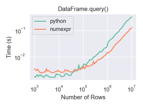
只有当您的框架行数超过大约 100,000 行时，您才能看到使用 numexpr 引擎配合 DataFrame.query() 带来的性能优势。

此图是使用一个包含 3 列的 DataFrame 创建的，每列都包含使用 numpy.random.randn() 生成的浮点值。

In [296]: df = pd.DataFrame(np.random.randn(8, 4),
   .....:                   index=dates, columns=['A', 'B', 'C', 'D'])
   .....: 

In [297]: df2 = df.copy()

重复数据#

如果您想识别并删除 DataFrame 中的重复行，有两个方法可以帮助您：duplicated 和 drop_duplicates。每个方法都接受用于识别重复行的列作为参数。

duplicated 返回一个布尔向量，其长度是行数，并指示一行是否重复。
drop_duplicates 删除重复行。

默认情况下，重复集中的第一个出现的行被认为是唯一的，但每个方法都有一个 keep 参数来指定要保留的目标。

keep='first'（默认）：标记/删除重复项，除了第一次出现。
keep='last'：标记/删除重复项，除了最后一次出现。
keep=False：标记/删除所有重复项。

In [298]: df2 = pd.DataFrame({'a': ['one', 'one', 'two', 'two', 'two', 'three', 'four'],
   .....:                     'b': ['x', 'y', 'x', 'y', 'x', 'x', 'x'],
   .....:                     'c': np.random.randn(7)})
   .....: 

In [299]: df2
Out[299]: 
       a  b         c
0    one  x -1.067137
1    one  y  0.309500
2    two  x -0.211056
3    two  y -1.842023
4    two  x -0.390820
5  three  x -1.964475
6   four  x  1.298329

In [300]: df2.duplicated('a')
Out[300]: 
0    False
1     True
2    False
3     True
4     True
5    False
6    False
dtype: bool

In [301]: df2.duplicated('a', keep='last')
Out[301]: 
0     True
1    False
2     True
3     True
4    False
5    False
6    False
dtype: bool

In [302]: df2.duplicated('a', keep=False)
Out[302]: 
0     True
1     True
2     True
3     True
4     True
5    False
6    False
dtype: bool

In [303]: df2.drop_duplicates('a')
Out[303]: 
       a  b         c
0    one  x -1.067137
2    two  x -0.211056
5  three  x -1.964475
6   four  x  1.298329

In [304]: df2.drop_duplicates('a', keep='last')
Out[304]: 
       a  b         c
1    one  y  0.309500
4    two  x -0.390820
5  three  x -1.964475
6   four  x  1.298329

In [305]: df2.drop_duplicates('a', keep=False)
Out[305]: 
       a  b         c
5  three  x -1.964475
6   four  x  1.298329

此外，您还可以传递列列表来识别重复项。

In [306]: df2.duplicated(['a', 'b'])
Out[306]: 
0    False
1    False
2    False
3    False
4     True
5    False
6    False
dtype: bool

In [307]: df2.drop_duplicates(['a', 'b'])
Out[307]: 
       a  b         c
0    one  x -1.067137
1    one  y  0.309500
2    two  x -0.211056
3    two  y -1.842023
5  three  x -1.964475
6   four  x  1.298329

要按索引值删除重复项，请使用 Index.duplicated 然后执行切片。keep 参数也提供相同的选项集。

In [308]: df3 = pd.DataFrame({'a': np.arange(6),
   .....:                     'b': np.random.randn(6)},
   .....:                    index=['a', 'a', 'b', 'c', 'b', 'a'])
   .....: 

In [309]: df3
Out[309]: 
   a         b
a  0  1.440455
a  1  2.456086
b  2  1.038402
c  3 -0.894409
b  4  0.683536
a  5  3.082764

In [310]: df3.index.duplicated()
Out[310]: array([False,  True, False, False,  True,  True])

In [311]: df3[~df3.index.duplicated()]
Out[311]: 
   a         b
a  0  1.440455
b  2  1.038402
c  3 -0.894409

In [312]: df3[~df3.index.duplicated(keep='last')]
Out[312]: 
   a         b
c  3 -0.894409
b  4  0.683536
a  5  3.082764

In [313]: df3[~df3.index.duplicated(keep=False)]
Out[313]: 
   a         b
c  3 -0.894409

字典风格的 `get()` 方法#

Series 或 DataFrame 都具有 get 方法，该方法可以返回默认值。

In [314]: s = pd.Series([1, 2, 3], index=['a', 'b', 'c'])

In [315]: s.get('a')  # equivalent to s['a']
Out[315]: 1

In [316]: s.get('x', default=-1)
Out[316]: -1

按索引/列标签查找值#

有时您希望根据一系列行标签和列标签提取一组值，这可以通过 pandas.factorize 和 NumPy 索引实现。例如

In [317]: df = pd.DataFrame({'col': ["A", "A", "B", "B"],
   .....:                    'A': [80, 23, np.nan, 22],
   .....:                    'B': [80, 55, 76, 67]})
   .....: 

In [318]: df
Out[318]: 
  col     A   B
0   A  80.0  80
1   A  23.0  55
2   B   NaN  76
3   B  22.0  67

In [319]: idx, cols = pd.factorize(df['col'])

In [320]: df.reindex(cols, axis=1).to_numpy()[np.arange(len(df)), idx]
Out[320]: array([80., 23., 76., 67.])

以前可以通过专门的 DataFrame.lookup 方法实现这一点，该方法在 1.2.0 版中已弃用，并在 2.0.0 版中移除。

Index 对象#

pandas 的 Index 类及其子类可以被视为实现了有序多重集。允许重复。

Index 还提供了查找、数据对齐和重新索引所需的基础设施。直接创建 Index 最简单的方法是将 list 或其他序列传递给 Index

In [321]: index = pd.Index(['e', 'd', 'a', 'b'])

In [322]: index
Out[322]: Index(['e', 'd', 'a', 'b'], dtype='object')

In [323]: 'd' in index
Out[323]: True

或使用数字

In [324]: index = pd.Index([1, 5, 12])

In [325]: index
Out[325]: Index([1, 5, 12], dtype='int64')

In [326]: 5 in index
Out[326]: True

如果未给定 dtype，Index 会尝试从数据中推断 dtype。在实例化 Index 时也可以指定显式 dtype。

In [327]: index = pd.Index(['e', 'd', 'a', 'b'], dtype="string")

In [328]: index
Out[328]: Index(['e', 'd', 'a', 'b'], dtype='string')

In [329]: index = pd.Index([1, 5, 12], dtype="int8")

In [330]: index
Out[330]: Index([1, 5, 12], dtype='int8')

In [331]: index = pd.Index([1, 5, 12], dtype="float32")

In [332]: index
Out[332]: Index([1.0, 5.0, 12.0], dtype='float32')

您还可以传递一个 name 以存储在索引中。

In [333]: index = pd.Index(['e', 'd', 'a', 'b'], name='something')

In [334]: index.name
Out[334]: 'something'

名称（如果已设置）将显示在控制台显示中。

In [335]: index = pd.Index(list(range(5)), name='rows')

In [336]: columns = pd.Index(['A', 'B', 'C'], name='cols')

In [337]: df = pd.DataFrame(np.random.randn(5, 3), index=index, columns=columns)

In [338]: df
Out[338]: 
cols         A         B         C
rows                              
0     1.295989 -1.051694  1.340429
1    -2.366110  0.428241  0.387275
2     0.433306  0.929548  0.278094
3     2.154730 -0.315628  0.264223
4     1.126818  1.132290 -0.353310

In [339]: df['A']
Out[339]: 
rows
0    1.295989
1   -2.366110
2    0.433306
3    2.154730
4    1.126818
Name: A, dtype: float64

设置元数据#

索引“大部分是不可变的”，但可以设置和更改它们的 name 属性。您可以使用 rename、set_names 直接设置这些属性，它们默认返回一个副本。

有关 MultiIndex 的用法，请参见高级索引。

In [340]: ind = pd.Index([1, 2, 3])

In [341]: ind.rename("apple")
Out[341]: Index([1, 2, 3], dtype='int64', name='apple')

In [342]: ind
Out[342]: Index([1, 2, 3], dtype='int64')

In [343]: ind = ind.set_names(["apple"])

In [344]: ind.name = "bob"

In [345]: ind
Out[345]: Index([1, 2, 3], dtype='int64', name='bob')

set_names、set_levels 和 set_codes 也接受一个可选的 level 参数。

In [346]: index = pd.MultiIndex.from_product([range(3), ['one', 'two']], names=['first', 'second'])

In [347]: index
Out[347]: 
MultiIndex([(0, 'one'),
            (0, 'two'),
            (1, 'one'),
            (1, 'two'),
            (2, 'one'),
            (2, 'two')],
           names=['first', 'second'])

In [348]: index.levels[1]
Out[348]: Index(['one', 'two'], dtype='object', name='second')

In [349]: index.set_levels(["a", "b"], level=1)
Out[349]: 
MultiIndex([(0, 'a'),
            (0, 'b'),
            (1, 'a'),
            (1, 'b'),
            (2, 'a'),
            (2, 'b')],
           names=['first', 'second'])

Index 对象的集合操作#

两个主要操作是 union 和 intersection。差集通过 .difference() 方法提供。

In [350]: a = pd.Index(['c', 'b', 'a'])

In [351]: b = pd.Index(['c', 'e', 'd'])

In [352]: a.difference(b)
Out[352]: Index(['a', 'b'], dtype='object')

还提供了 symmetric_difference 操作，它返回出现在 idx1 或 idx2 中但不同时出现在两者中的元素。这等同于由 idx1.difference(idx2).union(idx2.difference(idx1)) 创建的 Index，并去除了重复项。

In [353]: idx1 = pd.Index([1, 2, 3, 4])

In [354]: idx2 = pd.Index([2, 3, 4, 5])

In [355]: idx1.symmetric_difference(idx2)
Out[355]: Index([1, 5], dtype='int64')

注意

集合操作产生的索引将按升序排序。

当对不同 dtypes 的索引执行 Index.union() 操作时，索引必须转换为共同的 dtype。通常（但并非总是），这是 object dtype。例外情况是对整数和浮点数据执行联合操作时。在这种情况下，整数值会转换为浮点数。

In [356]: idx1 = pd.Index([0, 1, 2])

In [357]: idx2 = pd.Index([0.5, 1.5])

In [358]: idx1.union(idx2)
Out[358]: Index([0.0, 0.5, 1.0, 1.5, 2.0], dtype='float64')

缺失值#

重要

尽管 Index 可以包含缺失值 (NaN)，但如果您不希望出现任何意外结果，则应避免使用。例如，某些操作会隐式排除缺失值。

Index.fillna 使用指定的标量值填充缺失值。

In [359]: idx1 = pd.Index([1, np.nan, 3, 4])

In [360]: idx1
Out[360]: Index([1.0, nan, 3.0, 4.0], dtype='float64')

In [361]: idx1.fillna(2)
Out[361]: Index([1.0, 2.0, 3.0, 4.0], dtype='float64')

In [362]: idx2 = pd.DatetimeIndex([pd.Timestamp('2011-01-01'),
   .....:                          pd.NaT,
   .....:                          pd.Timestamp('2011-01-03')])
   .....: 

In [363]: idx2
Out[363]: DatetimeIndex(['2011-01-01', 'NaT', '2011-01-03'], dtype='datetime64[ns]', freq=None)

In [364]: idx2.fillna(pd.Timestamp('2011-01-02'))
Out[364]: DatetimeIndex(['2011-01-01', '2011-01-02', '2011-01-03'], dtype='datetime64[ns]', freq=None)

设置/重置索引#

有时您会将数据集加载或创建到 DataFrame 中，并希望在完成后添加索引。有几种不同的方法。

设置索引#

DataFrame 有一个 set_index() 方法，它接受一个列名（用于常规 Index）或列名列表（用于 MultiIndex）。要创建一个新的、重新索引的 DataFrame

In [365]: data = pd.DataFrame({'a': ['bar', 'bar', 'foo', 'foo'],
   .....:                      'b': ['one', 'two', 'one', 'two'],
   .....:                      'c': ['z', 'y', 'x', 'w'],
   .....:                      'd': [1., 2., 3, 4]})
   .....: 

In [366]: data
Out[366]: 
     a    b  c    d
0  bar  one  z  1.0
1  bar  two  y  2.0
2  foo  one  x  3.0
3  foo  two  w  4.0

In [367]: indexed1 = data.set_index('c')

In [368]: indexed1
Out[368]: 
     a    b    d
c               
z  bar  one  1.0
y  bar  two  2.0
x  foo  one  3.0
w  foo  two  4.0

In [369]: indexed2 = data.set_index(['a', 'b'])

In [370]: indexed2
Out[370]: 
         c    d
a   b          
bar one  z  1.0
    two  y  2.0
foo one  x  3.0
    two  w  4.0

append 关键字选项允许您保留现有索引并将给定列追加到 MultiIndex。

In [371]: frame = data.set_index('c', drop=False)

In [372]: frame = frame.set_index(['a', 'b'], append=True)

In [373]: frame
Out[373]: 
           c    d
c a   b          
z bar one  z  1.0
y bar two  y  2.0
x foo one  x  3.0
w foo two  w  4.0

set_index 中的其他选项允许您不删除索引列。

In [374]: data.set_index('c', drop=False)
Out[374]: 
     a    b  c    d
c                  
z  bar  one  z  1.0
y  bar  two  y  2.0
x  foo  one  x  3.0
w  foo  two  w  4.0

重置索引#

为了方便，DataFrame 上有一个新函数称为 reset_index()，它将索引值转移到 DataFrame 的列中并设置一个简单的整数索引。这是 set_index() 的逆操作。

In [375]: data
Out[375]: 
     a    b  c    d
0  bar  one  z  1.0
1  bar  two  y  2.0
2  foo  one  x  3.0
3  foo  two  w  4.0

In [376]: data.reset_index()
Out[376]: 
   index    a    b  c    d
0      0  bar  one  z  1.0
1      1  bar  two  y  2.0
2      2  foo  one  x  3.0
3      3  foo  two  w  4.0

输出更类似于 SQL 表或记录数组。从索引派生的列名是存储在 names 属性中的名称。

您可以使用 level 关键字仅删除索引的一部分。

In [377]: frame
Out[377]: 
           c    d
c a   b          
z bar one  z  1.0
y bar two  y  2.0
x foo one  x  3.0
w foo two  w  4.0

In [378]: frame.reset_index(level=1)
Out[378]: 
         a  c    d
c b               
z one  bar  z  1.0
y two  bar  y  2.0
x one  foo  x  3.0
w two  foo  w  4.0

reset_index 接受一个可选参数 drop，如果为 true，则简单地丢弃索引，而不是将索引值放入 DataFrame 的列中。

添加临时索引#

您可以将自定义索引赋值给 index 属性。

In [379]: df_idx = pd.DataFrame(range(4))

In [380]: df_idx.index = pd.Index([10, 20, 30, 40], name="a")

In [381]: df_idx
Out[381]: 
    0
a    
10  0
20  1
30  2
40  3

返回视图而非副本#

警告

写入时复制将成为 pandas 3.0 中的新默认行为。这意味着链式索引将永远无效。因此，SettingWithCopyWarning 将不再需要。有关更多背景信息，请参阅本节。我们建议启用写入时复制以利用以下改进：

` pd.options.mode.copy_on_write = True `

即使在 pandas 3.0 可用之前。

在 pandas 对象中设置值时，必须注意避免所谓的链式索引。这是一个示例。

In [382]: dfmi = pd.DataFrame([list('abcd'),
   .....:                      list('efgh'),
   .....:                      list('ijkl'),
   .....:                      list('mnop')],
   .....:                     columns=pd.MultiIndex.from_product([['one', 'two'],
   .....:                                                         ['first', 'second']]))
   .....: 

In [383]: dfmi
Out[383]: 
    one          two       
  first second first second
0     a      b     c      d
1     e      f     g      h
2     i      j     k      l
3     m      n     o      p

比较这两种访问方法

In [384]: dfmi['one']['second']
Out[384]: 
0    b
1    f
2    j
3    n
Name: second, dtype: object

In [385]: dfmi.loc[:, ('one', 'second')]
Out[385]: 
0    b
1    f
2    j
3    n
Name: (one, second), dtype: object

这两种方法都产生相同的结果，那么您应该使用哪一种呢？了解这些操作的顺序以及为什么方法 2（.loc）比方法 1（链式 []）更受青睐是很有启发性的。

dfmi['one'] 选择列的第一级并返回一个单索引的 DataFrame。然后另一个 Python 操作 dfmi_with_one['second'] 选择由 'second' 索引的 Series。这由变量 dfmi_with_one 表示，因为 pandas 将这些操作视为独立的事件，例如对 __getitem__ 的单独调用，因此它必须将它们视为线性操作，一个接一个地发生。

与此相反，df.loc[:,('one','second')] 将一个嵌套元组 (slice(None),('one','second')) 传递给 __getitem__ 的单个调用。这使得 pandas 能够将其作为一个单一实体处理。此外，这种操作顺序可能显着更快，并且如果需要，允许同时索引两个轴。

为什么使用链式索引时赋值会失败？#

警告

写入时复制将成为 pandas 3.0 中的新默认行为。这意味着链式索引将永远无效。因此，SettingWithCopyWarning 将不再需要。有关更多背景信息，请参阅本节。我们建议启用写入时复制以利用以下改进：

` pd.options.mode.copy_on_write = True `

即使在 pandas 3.0 可用之前。

上一节的问题只是性能问题。SettingWithCopy 警告是怎么回事？我们**通常**不会在您执行可能只花费几毫秒的操作时抛出警告！

但事实证明，赋值给链式索引的结果具有固有的不可预测性。要理解这一点，请思考 Python 解释器如何执行此代码：

dfmi.loc[:, ('one', 'second')] = value
# becomes
dfmi.loc.__setitem__((slice(None), ('one', 'second')), value)

但这段代码的处理方式不同：

dfmi['one']['second'] = value
# becomes
dfmi.__getitem__('one').__setitem__('second', value)

看到那里的 __getitem__ 了吗？除了简单的情况，很难预测它会返回视图还是副本（这取决于数组的内存布局，而 pandas 对此不作任何保证），因此 __setitem__ 是会修改 dfmi 还是修改一个随后立即丢弃的临时对象。**这就是** SettingWithCopy 警告您的内容！

注意

您可能想知道在第一个示例中是否应该关注 loc 属性。但是 dfmi.loc 保证是 dfmi 本身，具有修改后的索引行为，因此 dfmi.loc.__getitem__ / dfmi.loc.__setitem__ 直接作用于 dfmi。当然，dfmi.loc.__getitem__(idx) 可能是 dfmi 的视图或副本。

有时，即使没有明显的链式索引，也会出现 SettingWithCopy 警告。**这些**正是 SettingWithCopy 旨在捕获的错误！pandas 可能正在试图警告您您已经这样做了：

def do_something(df):
    foo = df[['bar', 'baz']]  # Is foo a view? A copy? Nobody knows!
    # ... many lines here ...
    # We don't know whether this will modify df or not!
    foo['quux'] = value
    return foo

哎呀！

求值顺序很重要#

警告

写入时复制将成为 pandas 3.0 中的新默认行为。这意味着链式索引将永远无效。因此，SettingWithCopyWarning 将不再需要。有关更多背景信息，请参阅本节。我们建议启用写入时复制以利用以下改进：

` pd.options.mode.copy_on_write = True `

即使在 pandas 3.0 可用之前。

当您使用链式索引时，索引操作的顺序和类型部分决定了结果是原始对象的切片，还是切片的副本。

pandas 之所以有 SettingWithCopyWarning，是因为赋值给切片的副本通常不是故意的，而是链式索引返回副本而期望切片所导致的错误。

如果您希望 pandas 对链式索引表达式的赋值更信任或不那么信任，您可以将选项 mode.chained_assignment 设置为以下值之一：

'warn'（默认值）表示会打印 SettingWithCopyWarning。
'raise' 表示 pandas 将引发 SettingWithCopyError，您必须处理它。
None 将完全抑制警告。

In [386]: dfb = pd.DataFrame({'a': ['one', 'one', 'two',
   .....:                           'three', 'two', 'one', 'six'],
   .....:                     'c': np.arange(7)})
   .....: 

# This will show the SettingWithCopyWarning
# but the frame values will be set
In [387]: dfb['c'][dfb['a'].str.startswith('o')] = 42

然而，这操作的是一个副本，因此无效。

In [388]: with pd.option_context('mode.chained_assignment','warn'):
   .....:     dfb[dfb['a'].str.startswith('o')]['c'] = 42
   .....: 

链式赋值也可能出现在混合 dtype 框架的设置中。

注意

这些设置规则适用于所有 .loc/.iloc。

以下是使用 .loc 访问多个项（使用 mask）和使用固定索引访问单个项的推荐方法：

In [389]: dfc = pd.DataFrame({'a': ['one', 'one', 'two',
   .....:                           'three', 'two', 'one', 'six'],
   .....:                     'c': np.arange(7)})
   .....: 

In [390]: dfd = dfc.copy()

# Setting multiple items using a mask
In [391]: mask = dfd['a'].str.startswith('o')

In [392]: dfd.loc[mask, 'c'] = 42

In [393]: dfd
Out[393]: 
       a   c
0    one  42
1    one  42
2    two   2
3  three   3
4    two   4
5    one  42
6    six   6

# Setting a single item
In [394]: dfd = dfc.copy()

In [395]: dfd.loc[2, 'a'] = 11

In [396]: dfd
Out[396]: 
       a  c
0    one  0
1    one  1
2     11  2
3  three  3
4    two  4
5    one  5
6    six  6

以下方法有时可能有效，但不能保证，因此应避免使用。

In [397]: dfd = dfc.copy()

In [398]: dfd['a'][2] = 111

In [399]: dfd
Out[399]: 
       a  c
0    one  0
1    one  1
2    111  2
3  three  3
4    two  4
5    one  5
6    six  6

最后，后续示例将完全**无效**，因此应避免使用。

In [400]: with pd.option_context('mode.chained_assignment','raise'):
   .....:     dfd.loc[0]['a'] = 1111
   .....: 
---------------------------------------------------------------------------
SettingWithCopyError                      Traceback (most recent call last)
<ipython-input-400-32ce785aaa5b> in ?()
      1 with pd.option_context('mode.chained_assignment','raise'):
----> 2     dfd.loc[0]['a'] = 1111

~/work/pandas/pandas/pandas/core/series.py in ?(self, key, value)
   1293                 )
   1294 
   1295         check_dict_or_set_indexers(key)
   1296         key = com.apply_if_callable(key, self)
-> 1297         cacher_needs_updating = self._check_is_chained_assignment_possible()
   1298 
   1299         if key is Ellipsis:
   1300             key = slice(None)

~/work/pandas/pandas/pandas/core/series.py in ?(self)
   1498             ref = self._get_cacher()
   1499             if ref is not None and ref._is_mixed_type:
   1500                 self._check_setitem_copy(t="referent", force=True)
   1501             return True
-> 1502         return super()._check_is_chained_assignment_possible()

~/work/pandas/pandas/pandas/core/generic.py in ?(self)
   4414         single-dtype meaning that the cacher should be updated following
   4415         setting.
   4416         """
   4417         if self._is_copy:
-> 4418             self._check_setitem_copy(t="referent")
   4419         return False

~/work/pandas/pandas/pandas/core/generic.py in ?(self, t, force)
   4488                 "indexing.html#returning-a-view-versus-a-copy"
   4489             )
   4490 
   4491         if value == "raise":
-> 4492             raise SettingWithCopyError(t)
   4493         if value == "warn":
   4494             warnings.warn(t, SettingWithCopyWarning, stacklevel=find_stack_level())

SettingWithCopyError: 
A value is trying to be set on a copy of a slice from a DataFrame

See the caveats in the documentation: https://pandas.ac.cn/pandas-docs/stable/user_guide/indexing.html#returning-a-view-versus-a-copy

警告

链式赋值警告/异常旨在告知用户可能无效的赋值。可能存在误报；即链式赋值被无意中报告的情况。

索引和选择数据#

不同的索引选择#

基础知识#

属性访问#

切片范围#

按标签选择#

按标签切片#

按位置选择#

按可调用对象选择#

结合位置和基于标签的索引#

重新索引#

选择随机样本#

伴随扩展的设置#

快速获取和设置标量值#

布尔索引#

使用 isin 进行索引#

where() 方法和掩码#

掩码#

使用 numpy() 有条件地进行扩展设置#

query() 方法#

MultiIndex query() 语法#

query() 用例#

query() Python 与 pandas 语法比较#

in 和 not in 运算符#

== 运算符与 list 对象的特殊用法#

布尔运算符#

query() 的性能#

重复数据#

字典风格的 get() 方法#

按索引/列标签查找值#

Index 对象#

设置元数据#

Index 对象的集合操作#

缺失值#

设置/重置索引#

设置索引#

重置索引#

添加临时索引#

返回视图而非副本#

为什么使用链式索引时赋值会失败？#

求值顺序很重要#

`where()` 方法和掩码#

使用 `numpy()` 有条件地进行扩展设置#

`query()` 方法#

`MultiIndex` `query()` 语法#

`query()` 用例#

`query()` Python 与 pandas 语法比较#

`in` 和 `not in` 运算符#

`==` 运算符与 `list` 对象的特殊用法#

`query()` 的性能#

字典风格的 `get()` 方法#