重塑和数据透视表#
pandas 提供了用于操作 Series 和 DataFrame 的方法,以改变数据表示形式,便于进一步的数据处理或数据汇总。
pivot()和pivot_table():将一个或多个离散类别中的唯一值分组。melt()和wide_to_long():将宽格式的DataFrame转换为长格式。get_dummies()和from_dummies():带有指示变量的转换。explode():将列中的列表状值转换为单独的行。crosstab():计算多个一维因子数组的交叉表。cut():将连续变量转换为离散的分类值factorize():将一维变量编码为整数标签。
pivot() 和 pivot_table()#
pivot()#
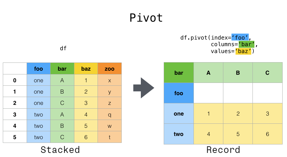
数据通常以所谓的“堆叠(stacked)”或“记录(record)”格式存储。在“记录”或“宽(wide)”格式中,通常每个主体对应一行。在“堆叠”或“长(long)”格式中,每个主体可能有多行。
In [1]: data = {
   ...:    "value": range(12),
   ...:    "variable": ["A"] * 3 + ["B"] * 3 + ["C"] * 3 + ["D"] * 3,
   ...:    "date": pd.to_datetime(["2020-01-03", "2020-01-04", "2020-01-05"] * 4)
   ...: }
   ...:

In [2]: df = pd.DataFrame(data)
为了对每个唯一变量执行时间序列操作,更好的表示形式是 columns 是唯一变量,并且日期的 index 标识了单个观测值。为了将数据重塑为这种形式,我们使用 DataFrame.pivot() 方法(也作为顶层函数 pivot())。
In [3]: pivoted = df.pivot(index="date", columns="variable", values="value")

In [4]: pivoted
Out[4]:
variable    A  B  C   D
date
2020-01-03  0  3  6   9
2020-01-04  1  4  7  10
2020-01-05  2  5  8  11
如果省略 values 参数,并且输入 DataFrame 有多个值列未用作列或索引输入到 pivot(),则生成的“透视” DataFrame 将具有 分层列,其最顶层指示相应的值列。
In [5]: df["value2"] = df["value"] * 2

In [6]: pivoted = df.pivot(index="date", columns="variable")

In [7]: pivoted
Out[7]:
           value           value2
variable       A  B  C   D      A   B   C   D
date
2020-01-03     0  3  6   9      0   6  12  18
2020-01-04     1  4  7  10      2   8  14  20
2020-01-05     2  5  8  11      4  10  16  22
然后您可以从透视后的 DataFrame 中选择子集。
In [8]: pivoted["value2"]
Out[8]:
variable    A   B   C   D
date
2020-01-03  0   6  12  18
2020-01-04  2   8  14  20
2020-01-05  4  10  16  22
请注意,在数据类型均匀的情况下,这会返回底层数据的视图。
注意
pivot() 只能处理由 index 和 columns 指定的唯一行。如果您的数据包含重复项,请使用 pivot_table()。
pivot_table()#
尽管 pivot() 提供了对各种数据类型的通用透视功能,pandas 还提供了 pivot_table() 或 pivot_table() 用于带有数值数据聚合的透视。
函数 pivot_table() 可用于创建电子表格样式的透视表。有关一些高级策略,请参阅 指南。
In [9]: import datetime

In [10]: df = pd.DataFrame(
   ....:     {
   ....:         "A": ["one", "one", "two", "three"] * 6,
   ....:         "B": ["A", "B", "C"] * 8,
   ....:         "C": ["foo", "foo", "foo", "bar", "bar", "bar"] * 4,
   ....:         "D": np.random.randn(24),
   ....:         "E": np.random.randn(24),
   ....:         "F": [datetime.datetime(2013, i, 1) for i in range(1, 13)]
   ....:         + [datetime.datetime(2013, i, 15) for i in range(1, 13)],
   ....:     }
   ....: )
   ....:

In [11]: df
Out[11]:
        A  B    C         D         E          F
0     one  A  foo  0.469112  0.404705 2013-01-01
1     one  B  foo -0.282863  0.577046 2013-02-01
2     two  C  foo -1.509059 -1.715002 2013-03-01
3   three  A  bar -1.135632 -1.039268 2013-04-01
4     one  B  bar  1.212112 -0.370647 2013-05-01
..    ... ..  ...       ...       ...        ...
19  three  B  foo -1.087401 -0.472035 2013-08-15
20    one  C  foo -0.673690 -0.013960 2013-09-15
21    one  A  bar  0.113648 -0.362543 2013-10-15
22    two  B  bar -1.478427 -0.006154 2013-11-15
23  three  C  bar  0.524988 -0.923061 2013-12-15

[24 rows x 6 columns]

In [12]: pd.pivot_table(df, values="D", index=["A", "B"], columns=["C"])
Out[12]:
C             bar       foo
A     B
one   A -0.995460  0.595334
      B  0.393570 -0.494817
      C  0.196903 -0.767769
three A -0.431886       NaN
      B       NaN -1.065818
      C  0.798396       NaN
two   A       NaN  0.197720
      B -0.986678       NaN
      C       NaN -1.274317

In [13]: pd.pivot_table(
   ....:     df, values=["D", "E"],
   ....:     index=["B"],
   ....:     columns=["A", "C"],
   ....:     aggfunc="sum",
   ....: )
   ....:
Out[13]:
          D                      ...         E
A       one               three  ...     three      two
C       bar       foo       bar  ...       foo      bar       foo
B                                ...
A -1.990921  1.190667 -0.863772  ...       NaN      NaN -1.067650
B  0.787140 -0.989634       NaN  ...  0.372851  1.63741       NaN
C  0.393806 -1.535539  1.596791  ...       NaN      NaN -3.491906

[3 rows x 12 columns]

In [14]: pd.pivot_table(
   ....:     df, values="E",
   ....:     index=["B", "C"],
   ....:     columns=["A"],
   ....:     aggfunc=["sum", "mean"],
   ....: )
   ....:
Out[14]:
            sum                          mean
A           one     three       two       one     three       two
B C
A bar -0.471593 -2.008182       NaN -0.235796 -1.004091       NaN
  foo  0.761726       NaN -1.067650  0.380863       NaN -0.533825
B bar -1.665170       NaN  1.637410 -0.832585       NaN  0.818705
  foo -0.097554  0.372851       NaN -0.048777  0.186425       NaN
C bar -0.744154 -2.392449       NaN -0.372077 -1.196224       NaN
  foo  1.061810       NaN -3.491906  0.530905       NaN -1.745953
结果是一个 DataFrame,可能在索引或列上具有 MultiIndex。如果未给定 values 列名,则透视表将在列中包含所有数据,作为额外的层次结构级别。
In [15]: pd.pivot_table(df[["A", "B", "C", "D", "E"]], index=["A", "B"], columns=["C"])
Out[15]:
                D                   E
C             bar       foo       bar       foo
A     B
one   A -0.995460  0.595334 -0.235796  0.380863
      B  0.393570 -0.494817 -0.832585 -0.048777
      C  0.196903 -0.767769 -0.372077  0.530905
three A -0.431886       NaN -1.004091       NaN
      B       NaN -1.065818       NaN  0.186425
      C  0.798396       NaN -1.196224       NaN
two   A       NaN  0.197720       NaN -0.533825
      B -0.986678       NaN  0.818705       NaN
      C       NaN -1.274317       NaN -1.745953
此外,您可以使用 Grouper 用于 index 和 columns 关键字。有关 Grouper 的详细信息,请参阅 使用 Grouper 规范进行分组。
In [16]: pd.pivot_table(df, values="D", index=pd.Grouper(freq="ME", key="F"), columns="C")
Out[16]:
C                bar       foo
F
2013-01-31       NaN  0.595334
2013-02-28       NaN -0.494817
2013-03-31       NaN -1.274317
2013-04-30 -0.431886       NaN
2013-05-31  0.393570       NaN
2013-06-30  0.196903       NaN
2013-07-31       NaN  0.197720
2013-08-31       NaN -1.065818
2013-09-30       NaN -0.767769
2013-10-31 -0.995460       NaN
2013-11-30 -0.986678       NaN
2013-12-31  0.798396       NaN
添加边距#
将 margins=True 传递给 pivot_table() 将在行和列中添加一个带有 All 标签的行和列,其中包含跨行和列类别的部分组聚合。
In [17]: table = df.pivot_table(
   ....:     index=["A", "B"],
   ....:     columns="C",
   ....:     values=["D", "E"],
   ....:     margins=True,
   ....:     aggfunc="std"
   ....: )
   ....:

In [18]: table
Out[18]:
                D                             E
C             bar       foo       All       bar       foo       All
A     B
one   A  1.568517  0.178504  1.293926  0.179247  0.033718  0.371275
      B  1.157593  0.299748  0.860059  0.653280  0.885047  0.779837
      C  0.523425  0.133049  0.638297  1.111310  0.770555  0.938819
three A  0.995247       NaN  0.995247  0.049748       NaN  0.049748
      B       NaN  0.030522  0.030522       NaN  0.931203  0.931203
      C  0.386657       NaN  0.386657  0.386312       NaN  0.386312
two   A       NaN  0.111032  0.111032       NaN  1.146201  1.146201
      B  0.695438       NaN  0.695438  1.166526       NaN  1.166526
      C       NaN  0.331975  0.331975       NaN  0.043771  0.043771
All      1.014073  0.713941  0.871016  0.881376  0.984017  0.923568
此外,您可以调用 DataFrame.stack() 以将透视后的 DataFrame 显示为具有多级索引。
In [19]: table.stack(future_stack=True)
Out[19]:
                  D         E
A   B C
one A bar  1.568517  0.179247
      foo  0.178504  0.033718
      All  1.293926  0.371275
    B bar  1.157593  0.653280
      foo  0.299748  0.885047
...             ...       ...
two C foo  0.331975  0.043771
      All  0.331975  0.043771
All   bar  1.014073  0.881376
      foo  0.713941  0.984017
      All  0.871016  0.923568

[30 rows x 2 columns]
stack() 和 unstack()#
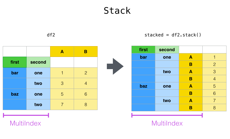
与 pivot() 方法密切相关的是适用于 Series 和 DataFrame 的相关 stack() 和 unstack() 方法。这些方法旨在与 MultiIndex 对象协同工作(请参阅有关 分层索引 的部分)。
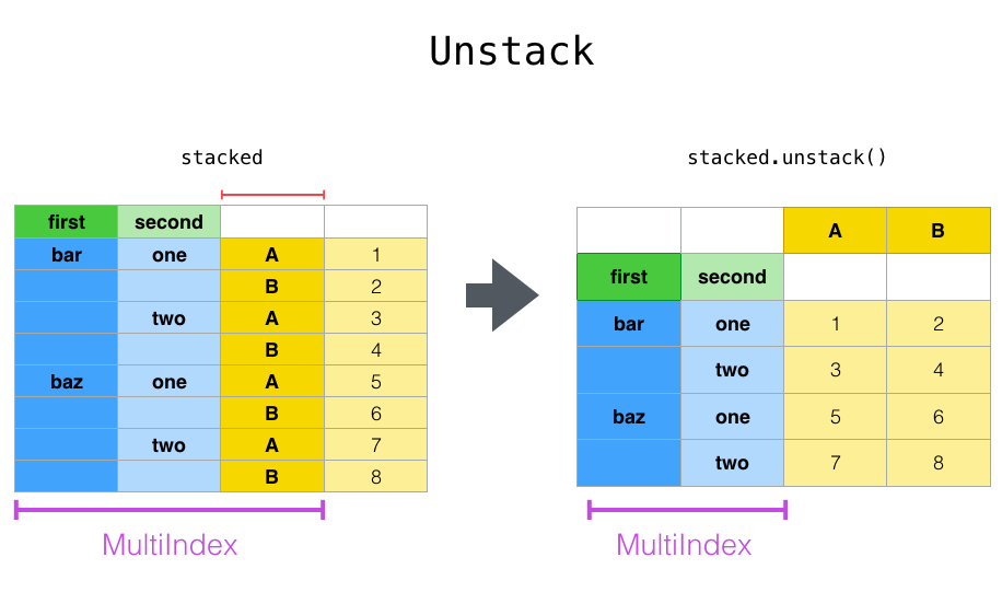
stack():将(可能是分层的)列标签的某一层“旋转”为行标签,返回一个索引具有新的最内层行标签的DataFrame。unstack():(是stack()的逆操作)将(可能是分层的)行索引的某一层“旋转”到列轴,生成一个重塑的DataFrame,其具有新的最内层列标签。
In [20]: tuples = [
   ....:    ["bar", "bar", "baz", "baz", "foo", "foo", "qux", "qux"],
   ....:    ["one", "two", "one", "two", "one", "two", "one", "two"],
   ....: ]
   ....:

In [21]: index = pd.MultiIndex.from_arrays(tuples, names=["first", "second"])

In [22]: df = pd.DataFrame(np.random.randn(8, 2), index=index, columns=["A", "B"])

In [23]: df2 = df[:4]

In [24]: df2
Out[24]:
                     A         B
first second
bar   one     0.895717  0.805244
      two    -1.206412  2.565646
baz   one     1.431256  1.340309
      two    -1.170299 -0.226169
函数 stack() “压缩”了 DataFrame 列中的一个级别,以生成以下之一:
一个
DataFrame,当列中存在MultiIndex时。
如果列具有 MultiIndex,您可以选择要堆叠的级别。堆叠后的级别将成为列中 MultiIndex 的新的最低级别。
In [25]: stacked = df2.stack(future_stack=True)

In [26]: stacked
Out[26]:
first  second
bar    one     A    0.895717
               B    0.805244
       two     A   -1.206412
               B    2.565646
baz    one     A    1.431256
               B    1.340309
       two     A   -1.170299
               B   -0.226169
dtype: float64
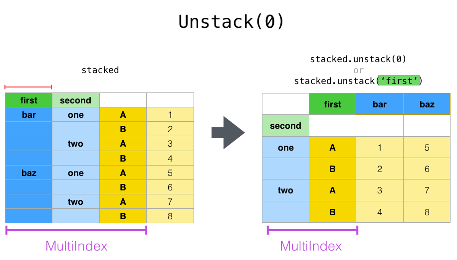
对于一个“堆叠”的 DataFrame 或 Series(其 MultiIndex 作为 index), stack() 的逆操作是 unstack(),它默认解除堆叠 最后一个级别。
In [27]: stacked.unstack()
Out[27]:
                     A         B
first second
bar   one     0.895717  0.805244
      two    -1.206412  2.565646
baz   one     1.431256  1.340309
      two    -1.170299 -0.226169

In [28]: stacked.unstack(1)
Out[28]:
second        one       two
first
bar   A  0.895717 -1.206412
      B  0.805244  2.565646
baz   A  1.431256 -1.170299
      B  1.340309 -0.226169

In [29]: stacked.unstack(0)
Out[29]:
first          bar       baz
second
one    A  0.895717  1.431256
       B  0.805244  1.340309
two    A -1.206412 -1.170299
       B  2.565646 -0.226169
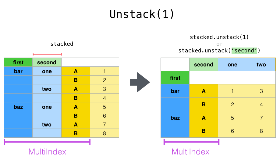
如果索引有名称,您可以使用级别名称而不是指定级别编号。
In [30]: stacked.unstack("second")
Out[30]:
second        one       two
first
bar   A  0.895717 -1.206412
      B  0.805244  2.565646
baz   A  1.431256 -1.170299
      B  1.340309 -0.226169
请注意, stack() 和 unstack() 方法会隐式地对涉及的索引级别进行排序。因此,调用 stack() 然后 unstack(),反之亦然,将导致原始 DataFrame 或 Series 的 已排序 副本。
In [31]: index = pd.MultiIndex.from_product([[2, 1], ["a", "b"]])

In [32]: df = pd.DataFrame(np.random.randn(4), index=index, columns=["A"])

In [33]: df
Out[33]:
            A
2 a -1.413681
  b  1.607920
1 a  1.024180
  b  0.569605

In [34]: all(df.unstack().stack(future_stack=True) == df.sort_index())
Out[34]: True
多个级别#
您还可以通过传递一个级别列表来一次堆叠或解除堆叠多个级别,在这种情况下,最终结果就像列表中每个级别都单独处理了一样。
In [35]: columns = pd.MultiIndex.from_tuples(
   ....:     [
   ....:         ("A", "cat", "long"),
   ....:         ("B", "cat", "long"),
   ....:         ("A", "dog", "short"),
   ....:         ("B", "dog", "short"),
   ....:     ],
   ....:     names=["exp", "animal", "hair_length"],
   ....: )
   ....:

In [36]: df = pd.DataFrame(np.random.randn(4, 4), columns=columns)

In [37]: df
Out[37]:
exp                 A         B         A         B
animal            cat       cat       dog       dog
hair_length      long      long     short     short
0            0.875906 -2.211372  0.974466 -2.006747
1           -0.410001 -0.078638  0.545952 -1.219217
2           -1.226825  0.769804 -1.281247 -0.727707
3           -0.121306 -0.097883  0.695775  0.341734

In [38]: df.stack(level=["animal", "hair_length"], future_stack=True)
Out[38]:
exp                          A         B
  animal hair_length
0 cat    long         0.875906 -2.211372
  dog    short        0.974466 -2.006747
1 cat    long        -0.410001 -0.078638
  dog    short        0.545952 -1.219217
2 cat    long        -1.226825  0.769804
  dog    short       -1.281247 -0.727707
3 cat    long        -0.121306 -0.097883
  dog    short        0.695775  0.341734
级别列表可以包含级别名称或级别编号,但不能混合使用两者。
# df.stack(level=['animal', 'hair_length'], future_stack=True)
# from above is equivalent to:
In [39]: df.stack(level=[1, 2], future_stack=True)
Out[39]:
exp                          A         B
  animal hair_length
0 cat    long         0.875906 -2.211372
  dog    short        0.974466 -2.006747
1 cat    long        -0.410001 -0.078638
  dog    short        0.545952 -1.219217
2 cat    long        -1.226825  0.769804
  dog    short       -1.281247 -0.727707
3 cat    long        -0.121306 -0.097883
  dog    short        0.695775  0.341734
缺失数据#
如果子组没有相同的标签集,解除堆叠可能会导致缺失值。默认情况下,缺失值将替换为该数据类型的默认填充值。
In [40]: columns = pd.MultiIndex.from_tuples(
   ....:     [
   ....:         ("A", "cat"),
   ....:         ("B", "dog"),
   ....:         ("B", "cat"),
   ....:         ("A", "dog"),
   ....:     ],
   ....:     names=["exp", "animal"],
   ....: )
   ....:

In [41]: index = pd.MultiIndex.from_product(
   ....:     [("bar", "baz", "foo", "qux"), ("one", "two")], names=["first", "second"]
   ....: )
   ....:

In [42]: df = pd.DataFrame(np.random.randn(8, 4), index=index, columns=columns)

In [43]: df3 = df.iloc[[0, 1, 4, 7], [1, 2]]

In [44]: df3
Out[44]:
exp                  B
animal             dog       cat
first second
bar   one    -1.110336 -0.619976
      two     0.687738  0.176444
foo   one     1.314232  0.690579
qux   two     0.380396  0.084844

In [45]: df3.unstack()
Out[45]:
exp            B
animal       dog                 cat
second       one       two       one       two
first
bar    -1.110336  0.687738 -0.619976  0.176444
foo     1.314232       NaN  0.690579       NaN
qux          NaN  0.380396       NaN  0.084844
缺失值可以通过 fill_value 参数填充为特定值。
In [46]: df3.unstack(fill_value=-1e9)
Out[46]:
exp                B
animal           dog                         cat
second           one           two           one           two
first
bar    -1.110336e+00  6.877384e-01 -6.199759e-01  1.764443e-01
foo     1.314232e+00 -1.000000e+09  6.905793e-01 -1.000000e+09
qux    -1.000000e+09  3.803956e-01 -1.000000e+09  8.484421e-02
melt() 和 wide_to_long()#
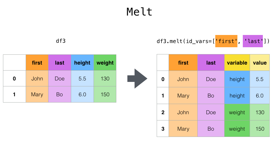
顶层 melt() 函数和相应的 DataFrame.melt() 有助于将 DataFrame 整理成一种格式,其中一个或多个列是标识符变量,而所有其他被视为测量变量的列则“解除透视”到行轴,只剩下两个非标识符列:“variable”和“value”。这些列的名称可以通过提供 var_name 和 value_name 参数进行自定义。
In [47]: cheese = pd.DataFrame(
   ....:     {
   ....:         "first": ["John", "Mary"],
   ....:         "last": ["Doe", "Bo"],
   ....:         "height": [5.5, 6.0],
   ....:         "weight": [130, 150],
   ....:     }
   ....: )
   ....:

In [48]: cheese
Out[48]:
  first last  height  weight
0  John  Doe     5.5     130
1  Mary   Bo     6.0     150

In [49]: cheese.melt(id_vars=["first", "last"])
Out[49]:
  first last variable  value
0  John  Doe   height    5.5
1  Mary   Bo   height    6.0
2  John  Doe   weight  130.0
3  Mary   Bo   weight  150.0

In [50]: cheese.melt(id_vars=["first", "last"], var_name="quantity")
Out[50]:
  first last quantity  value
0  John  Doe   height    5.5
1  Mary   Bo   height    6.0
2  John  Doe   weight  130.0
3  Mary   Bo   weight  150.0
当使用 melt() 转换 DataFrame 时,索引将被忽略。通过将 ignore_index=False 参数设置为 False(默认是 True),可以保留原始索引值。然而,ignore_index=False 会导致索引值重复。
In [51]: index = pd.MultiIndex.from_tuples([("person", "A"), ("person", "B")])

In [52]: cheese = pd.DataFrame(
   ....:     {
   ....:         "first": ["John", "Mary"],
   ....:         "last": ["Doe", "Bo"],
   ....:         "height": [5.5, 6.0],
   ....:         "weight": [130, 150],
   ....:     },
   ....:     index=index,
   ....: )
   ....:

In [53]: cheese
Out[53]:
         first last  height  weight
person A  John  Doe     5.5     130
       B  Mary   Bo     6.0     150

In [54]: cheese.melt(id_vars=["first", "last"])
Out[54]:
  first last variable  value
0  John  Doe   height    5.5
1  Mary   Bo   height    6.0
2  John  Doe   weight  130.0
3  Mary   Bo   weight  150.0

In [55]: cheese.melt(id_vars=["first", "last"], ignore_index=False)
Out[55]:
         first last variable  value
person A  John  Doe   height    5.5
       B  Mary   Bo   height    6.0
       A  John  Doe   weight  130.0
       B  Mary   Bo   weight  150.0
wide_to_long() 与 melt() 类似,但提供了更多的列匹配自定义功能。
In [56]: dft = pd.DataFrame(
   ....:     {
   ....:         "A1970": {0: "a", 1: "b", 2: "c"},
   ....:         "A1980": {0: "d", 1: "e", 2: "f"},
   ....:         "B1970": {0: 2.5, 1: 1.2, 2: 0.7},
   ....:         "B1980": {0: 3.2, 1: 1.3, 2: 0.1},
   ....:         "X": dict(zip(range(3), np.random.randn(3))),
   ....:     }
   ....: )
   ....:

In [57]: dft["id"] = dft.index

In [58]: dft
Out[58]:
  A1970 A1980  B1970  B1980         X  id
0     a     d    2.5    3.2  1.519970   0
1     b     e    1.2    1.3 -0.493662   1
2     c     f    0.7    0.1  0.600178   2

In [59]: pd.wide_to_long(dft, ["A", "B"], i="id", j="year")
Out[59]:
                X  A    B
id year
0  1970  1.519970  a  2.5
1  1970 -0.493662  b  1.2
2  1970  0.600178  c  0.7
0  1980  1.519970  d  3.2
1  1980 -0.493662  e  1.3
2  1980  0.600178  f  0.1
get_dummies() 和 from_dummies()#
为了将 Series 的分类变量转换为“虚拟(dummy)”或“指示符(indicator)”变量, get_dummies() 会创建一个新的 DataFrame,其列是唯一变量,值表示每行中这些变量的存在。
In [60]: df = pd.DataFrame({"key": list("bbacab"), "data1": range(6)})

In [61]: pd.get_dummies(df["key"])
Out[61]:
       a      b      c
0  False   True  False
1  False   True  False
2   True  False  False
3  False  False   True
4   True  False  False
5  False   True  False

In [62]: df["key"].str.get_dummies()
Out[62]:
   a  b  c
0  0  1  0
1  0  1  0
2  1  0  0
3  0  0  1
4  1  0  0
5  0  1  0
prefix 为列名添加一个前缀,这对于将结果与原始 DataFrame 合并很有用。
In [63]: dummies = pd.get_dummies(df["key"], prefix="key")

In [64]: dummies
Out[64]:
   key_a  key_b  key_c
0  False   True  False
1  False   True  False
2   True  False  False
3  False  False   True
4   True  False  False
5  False   True  False

In [65]: df[["data1"]].join(dummies)
Out[65]:
   data1  key_a  key_b  key_c
0      0  False   True  False
1      1  False   True  False
2      2   True  False  False
3      3  False  False   True
4      4   True  False  False
5      5  False   True  False
此函数通常与诸如 cut() 之类的离散化函数一起使用。
In [66]: values = np.random.randn(10)

In [67]: values
Out[67]:
array([ 0.2742,  0.1329, -0.0237,  2.4102,  1.4505,  0.2061, -0.2519,
       -2.2136,  1.0633,  1.2661])

In [68]: bins = [0, 0.2, 0.4, 0.6, 0.8, 1]

In [69]: pd.get_dummies(pd.cut(values, bins))
Out[69]:
   (0.0, 0.2]  (0.2, 0.4]  (0.4, 0.6]  (0.6, 0.8]  (0.8, 1.0]
0       False        True       False       False       False
1        True       False       False       False       False
2       False       False       False       False       False
3       False       False       False       False       False
4       False       False       False       False       False
5       False        True       False       False       False
6       False       False       False       False       False
7       False       False       False       False       False
8       False       False       False       False       False
9       False       False       False       False       False
get_dummies() 也接受一个 DataFrame。默认情况下,object、string 或 categorical 类型的列被编码为虚拟变量,其他列保持不变。
In [70]: df = pd.DataFrame({"A": ["a", "b", "a"], "B": ["c", "c", "b"], "C": [1, 2, 3]})

In [71]: pd.get_dummies(df)
Out[71]:
   C    A_a    A_b    B_b    B_c
0  1   True  False  False   True
1  2  False   True  False   True
2  3   True  False   True  False
指定 columns 关键字将编码任何类型的列。
In [72]: pd.get_dummies(df, columns=["A"])
Out[72]:
   B  C    A_a    A_b
0  c  1   True  False
1  c  2  False   True
2  b  3   True  False
与 Series 版本一样,您可以为 prefix 和 prefix_sep 传递值。默认情况下,列名用作前缀,_ 用作前缀分隔符。您可以通过3种方式指定 prefix 和 prefix_sep:
字符串:对要编码的每列使用相同的值作为
prefix或prefix_sep。列表:必须与要编码的列数长度相同。
字典:将列名映射到前缀。
In [73]: simple = pd.get_dummies(df, prefix="new_prefix")

In [74]: simple
Out[74]:
   C  new_prefix_a  new_prefix_b  new_prefix_b  new_prefix_c
0  1          True         False         False          True
1  2         False          True         False          True
2  3          True         False          True         False

In [75]: from_list = pd.get_dummies(df, prefix=["from_A", "from_B"])

In [76]: from_list
Out[76]:
   C  from_A_a  from_A_b  from_B_b  from_B_c
0  1      True     False     False      True
1  2     False      True     False      True
2  3      True     False      True     False

In [77]: from_dict = pd.get_dummies(df, prefix={"B": "from_B", "A": "from_A"})

In [78]: from_dict
Out[78]:
   C  from_A_a  from_A_b  from_B_b  from_B_c
0  1      True     False     False      True
1  2     False      True     False      True
2  3      True     False      True     False
为了避免将结果输入统计模型时出现共线性,请指定 drop_first=True。
In [79]: s = pd.Series(list("abcaa"))

In [80]: pd.get_dummies(s)
Out[80]:
       a      b      c
0   True  False  False
1  False   True  False
2  False  False   True
3   True  False  False
4   True  False  False

In [81]: pd.get_dummies(s, drop_first=True)
Out[81]:
       b      c
0  False  False
1   True  False
2  False   True
3  False  False
4  False  False
当列只包含一个级别时,它将在结果中被省略。
In [82]: df = pd.DataFrame({"A": list("aaaaa"), "B": list("ababc")})

In [83]: pd.get_dummies(df)
Out[83]:
    A_a    B_a    B_b    B_c
0  True   True  False  False
1  True  False   True  False
2  True   True  False  False
3  True  False   True  False
4  True  False  False   True

In [84]: pd.get_dummies(df, drop_first=True)
Out[84]:
     B_b    B_c
0  False  False
1   True  False
2  False  False
3   True  False
4  False   True
值可以使用 dtype 参数转换为不同的类型。
In [85]: df = pd.DataFrame({"A": list("abc"), "B": [1.1, 2.2, 3.3]})

In [86]: pd.get_dummies(df, dtype=np.float32).dtypes
Out[86]:
B      float64
A_a    float32
A_b    float32
A_c    float32
dtype: object
在 1.5.0 版中新增。
from_dummies() 将 get_dummies() 的输出从指示符值转换回分类值的 Series。
In [87]: df = pd.DataFrame({"prefix_a": [0, 1, 0], "prefix_b": [1, 0, 1]})

In [88]: df
Out[88]:
   prefix_a  prefix_b
0         0         1
1         1         0
2         0         1

In [89]: pd.from_dummies(df, sep="_")
Out[89]:
  prefix
0      b
1      a
2      b
虚拟编码的数据只需要包含 k - 1 个类别,在这种情况下,最后一个类别是默认类别。默认类别可以通过 default_category 进行修改。
In [90]: df = pd.DataFrame({"prefix_a": [0, 1, 0]})

In [91]: df
Out[91]:
   prefix_a
0         0
1         1
2         0

In [92]: pd.from_dummies(df, sep="_", default_category="b")
Out[92]:
  prefix
0      b
1      a
2      b
explode()#
对于一个 DataFrame 具有嵌套、列表状值的列, explode() 会将每个列表状值转换为单独的行。结果 Index 将根据原始行的索引标签进行复制。
In [93]: keys = ["panda1", "panda2", "panda3"]

In [94]: values = [["eats", "shoots"], ["shoots", "leaves"], ["eats", "leaves"]]

In [95]: df = pd.DataFrame({"keys": keys, "values": values})

In [96]: df
Out[96]:
     keys            values
0  panda1    [eats, shoots]
1  panda2  [shoots, leaves]
2  panda3    [eats, leaves]

In [97]: df["values"].explode()
Out[97]:
0      eats
0    shoots
1    shoots
1    leaves
2      eats
2    leaves
Name: values, dtype: object
DataFrame.explode 也可以在 DataFrame 中展开列。
In [98]: df.explode("values")
Out[98]:
     keys  values
0  panda1    eats
0  panda1  shoots
1  panda2  shoots
1  panda2  leaves
2  panda3    eats
2  panda3  leaves
Series.explode() 会将空列表替换为缺失值指示符,并保留标量条目。
In [99]: s = pd.Series([[1, 2, 3], "foo", [], ["a", "b"]])

In [100]: s
Out[100]:
0    [1, 2, 3]
1          foo
2           []
3       [a, b]
dtype: object

In [101]: s.explode()
Out[101]:
0      1
0      2
0      3
1    foo
2    NaN
3      a
3      b
dtype: object
逗号分隔的字符串值可以拆分为列表中的单个值,然后展开为新行。
In [102]: df = pd.DataFrame([{"var1": "a,b,c", "var2": 1}, {"var1": "d,e,f", "var2": 2}])

In [103]: df.assign(var1=df.var1.str.split(",")).explode("var1")
Out[103]:
  var1  var2
0    a     1
0    b     1
0    c     1
1    d     2
1    e     2
1    f     2
crosstab()#
使用 crosstab() 来计算两个(或更多)因子的交叉表。默认情况下, crosstab() 会计算因子的频率表,除非传入一个值数组和聚合函数。
任何传入的 Series 都将使用其名称属性,除非为交叉表指定了行或列名称。
In [104]: a = np.array(["foo", "foo", "bar", "bar", "foo", "foo"], dtype=object)

In [105]: b = np.array(["one", "one", "two", "one", "two", "one"], dtype=object)

In [106]: c = np.array(["dull", "dull", "shiny", "dull", "dull", "shiny"], dtype=object)

In [107]: pd.crosstab(a, [b, c], rownames=["a"], colnames=["b", "c"])
Out[107]:
b    one        two
c   dull shiny dull shiny
a
bar    1     0    0     1
foo    2     1    1     0
如果 crosstab() 只接收两个 Series,它将提供一个频率表。
In [108]: df = pd.DataFrame(
   .....:     {"A": [1, 2, 2, 2, 2], "B": [3, 3, 4, 4, 4], "C": [1, 1, np.nan, 1, 1]}
   .....: )
   .....:

In [109]: df
Out[109]:
   A  B    C
0  1  3  1.0
1  2  3  1.0
2  2  4  NaN
3  2  4  1.0
4  2  4  1.0

In [110]: pd.crosstab(df["A"], df["B"])
Out[110]:
B  3  4
A
1  1  0
2  1  3
crosstab() 还可以汇总为 Categorical 数据。
In [111]: foo = pd.Categorical(["a", "b"], categories=["a", "b", "c"])

In [112]: bar = pd.Categorical(["d", "e"], categories=["d", "e", "f"])

In [113]: pd.crosstab(foo, bar)
Out[113]:
col_0  d  e
row_0
a      1  0
b      0  1
对于 Categorical 数据,即使实际数据不包含特定类别的任何实例,若要包含 所有 数据类别,请使用 dropna=False。
In [114]: pd.crosstab(foo, bar, dropna=False)
Out[114]:
col_0  d  e  f
row_0
a      1  0  0
b      0  1  0
c      0  0  0
归一化#
频率表也可以使用 normalize 参数进行归一化,以显示百分比而非计数。
In [115]: pd.crosstab(df["A"], df["B"], normalize=True)
Out[115]:
B    3    4
A
1  0.2  0.0
2  0.2  0.6
normalize 还可以对每行或每列中的值进行归一化。
In [116]: pd.crosstab(df["A"], df["B"], normalize="columns")
Out[116]:
B    3    4
A
1  0.5  0.0
2  0.5  1.0
crosstab() 还可以接受第三个 Series 和一个聚合函数(aggfunc),该函数将应用于由前两个 Series 定义的每个组中第三个 Series 的值。
In [117]: pd.crosstab(df["A"], df["B"], values=df["C"], aggfunc="sum")
Out[117]:
B    3    4
A
1  1.0  NaN
2  1.0  2.0
添加边距#
margins=True 将在行和列中添加一个带有 All 标签的行和列,其中包含跨行和列类别的部分组聚合。
In [118]: pd.crosstab(
   .....:     df["A"], df["B"], values=df["C"], aggfunc="sum", normalize=True, margins=True
   .....: )
   .....:
Out[118]:
B       3    4   All
A
1    0.25  0.0  0.25
2    0.25  0.5  0.75
All  0.50  0.5  1.00
cut()#
函数 cut() 计算输入数组值的分组,并常用于将连续变量转换为离散或分类变量。
一个整数 bins 将形成等宽的箱。
In [119]: ages = np.array([10, 15, 13, 12, 23, 25, 28, 59, 60])

In [120]: pd.cut(ages, bins=3)
Out[120]:
[(9.95, 26.667], (9.95, 26.667], (9.95, 26.667], (9.95, 26.667], (9.95, 26.667], (9.95, 26.667], (26.667, 43.333], (43.333, 60.0], (43.333, 60.0]]
Categories (3, interval[float64, right]): [(9.95, 26.667] < (26.667, 43.333] < (43.333, 60.0]]
有序的箱边列表将为每个变量分配一个区间。
In [121]: pd.cut(ages, bins=[0, 18, 35, 70])
Out[121]:
[(0, 18], (0, 18], (0, 18], (0, 18], (18, 35], (18, 35], (18, 35], (35, 70], (35, 70]]
Categories (3, interval[int64, right]): [(0, 18] < (18, 35] < (35, 70]]
如果 bins 关键字是一个 IntervalIndex,那么这些将被用来对传入的数据进行分箱。
In [122]: pd.cut(ages, bins=pd.IntervalIndex.from_breaks([0, 40, 70]))
Out[122]:
[(0, 40], (0, 40], (0, 40], (0, 40], (0, 40], (0, 40], (0, 40], (40, 70], (40, 70]]
Categories (2, interval[int64, right]): [(0, 40] < (40, 70]]
factorize()#
factorize() 将一维值编码为整数标签。缺失值被编码为 -1。
In [123]: x = pd.Series(["A", "A", np.nan, "B", 3.14, np.inf])

In [124]: x
Out[124]:
0       A
1       A
2     NaN
3       B
4    3.14
5     inf
dtype: object

In [125]: labels, uniques = pd.factorize(x)

In [126]: labels
Out[126]: array([ 0,  0, -1,  1,  2,  3])

In [127]: uniques
Out[127]: Index(['A', 'B', 3.14, inf], dtype='object')
Categorical 也将类似地编码一维值,以进行进一步的分类操作。
In [128]: pd.Categorical(x)
Out[128]:
['A', 'A', NaN, 'B', 3.14, inf]
Categories (4, object): [3.14, inf, 'A', 'B']