In [1]: import pandas as pd

In [2]: import matplotlib.pyplot as plt
-
空气质量数据
In [3]: air_quality = pd.read_csv("data/air_quality_no2_long.csv")

In [4]: air_quality = air_quality.rename(columns={"date.utc": "datetime"})

In [5]: air_quality.head()
Out[5]:
    city country                   datetime location parameter  value   unit
0  Paris      FR  2019-06-21 00:00:00+00:00  FR04014       no2   20.0  µg/m³
1  Paris      FR  2019-06-20 23:00:00+00:00  FR04014       no2   21.8  µg/m³
2  Paris      FR  2019-06-20 22:00:00+00:00  FR04014       no2   26.5  µg/m³
3  Paris      FR  2019-06-20 21:00:00+00:00  FR04014       no2   24.9  µg/m³
4  Paris      FR  2019-06-20 20:00:00+00:00  FR04014       no2   21.4  µg/m³
In [6]: air_quality.city.unique()
Out[6]: array(['Paris', 'Antwerpen', 'London'], dtype=object)
如何轻松处理时间序列数据#
使用 pandas 日期时间属性#
我想将
datetime列中的日期作为日期时间对象而不是纯文本来处理In [7]: air_quality["datetime"] = pd.to_datetime(air_quality["datetime"]) In [8]: air_quality["datetime"] Out[8]: 0 2019-06-21 00:00:00+00:00 1 2019-06-20 23:00:00+00:00 2 2019-06-20 22:00:00+00:00 3 2019-06-20 21:00:00+00:00 4 2019-06-20 20:00:00+00:00 ... 2063 2019-05-07 06:00:00+00:00 2064 2019-05-07 04:00:00+00:00 2065 2019-05-07 03:00:00+00:00 2066 2019-05-07 02:00:00+00:00 2067 2019-05-07 01:00:00+00:00 Name: datetime, Length: 2068, dtype: datetime64[ns, UTC]
最初,
datetime中的值是字符串,不提供任何日期时间操作(例如,提取年份、星期几等)。通过应用to_datetime函数,pandas 会解释这些字符串并将其转换为日期时间(即datetime64[ns, UTC])对象。在 pandas 中,我们将这些日期时间对象称为pandas.Timestamp,类似于标准库中的datetime.datetime。
注意
由于许多数据集的列中包含日期时间信息,pandas 的输入函数如 pandas.read_csv() 和 pandas.read_json() 可以在读取数据时,使用 parse_dates 参数(提供要作为 Timestamp 读取的列列表)来完成日期的转换。
pd.read_csv("../data/air_quality_no2_long.csv", parse_dates=["datetime"])
为什么这些 pandas.Timestamp 对象很有用?让我们通过一些示例来 H 说明其附加价值。
我们正在处理的时间序列数据集的开始和结束日期是什么?
In [9]: air_quality["datetime"].min(), air_quality["datetime"].max()
Out[9]:
(Timestamp('2019-05-07 01:00:00+0000', tz='UTC'),
 Timestamp('2019-06-21 00:00:00+0000', tz='UTC'))
使用 pandas.Timestamp 处理日期时间使我们能够使用日期信息进行计算并使其具有可比性。因此,我们可以用它来获取时间序列的长度
In [10]: air_quality["datetime"].max() - air_quality["datetime"].min()
Out[10]: Timedelta('44 days 23:00:00')
结果是一个 pandas.Timedelta 对象,类似于标准 Python 库中的 datetime.timedelta,它定义了一个时间持续期。
pandas 支持的各种时间概念在用户指南的 时间相关概念 部分进行了解释。
我想向
DataFrame添加一个新列,其中只包含测量月份In [11]: air_quality["month"] = air_quality["datetime"].dt.month In [12]: air_quality.head() Out[12]: city country datetime ... value unit month 0 Paris FR 2019-06-21 00:00:00+00:00 ... 20.0 µg/m³ 6 1 Paris FR 2019-06-20 23:00:00+00:00 ... 21.8 µg/m³ 6 2 Paris FR 2019-06-20 22:00:00+00:00 ... 26.5 µg/m³ 6 3 Paris FR 2019-06-20 21:00:00+00:00 ... 24.9 µg/m³ 6 4 Paris FR 2019-06-20 20:00:00+00:00 ... 21.4 µg/m³ 6 [5 rows x 8 columns]
通过对日期使用
Timestamp对象,pandas 提供了许多时间相关属性。例如month,还有year、quarter等。所有这些属性都可以通过dt访问器访问。
现有日期属性的概述在时间和日期组件概览表中给出。关于 dt 访问器返回日期时间类属性的更多详细信息在dt 访问器的专门章节中进行了解释。
每个测量地点每周每一天的平均 \(NO_2\) 浓度是多少?
In [13]: air_quality.groupby(
   ....:     [air_quality["datetime"].dt.weekday, "location"])["value"].mean()
   ....:
Out[13]:
datetime  location
0         BETR801               27.875000
          FR04014               24.856250
          London Westminster    23.969697
1         BETR801               22.214286
          FR04014               30.999359
                                  ...
5         FR04014               25.266154
          London Westminster    24.977612
6         BETR801               21.896552
          FR04014               23.274306
          London Westminster    24.859155
Name: value, Length: 21, dtype: float64
还记得统计计算教程中
groupby提供的“拆分-应用-合并”模式吗?在这里,我们希望计算给定统计量(例如平均 \(NO_2\))**对于每周的每一天**以及**对于每个测量地点**。为了按工作日分组,我们使用 pandasTimestamp的日期时间属性weekday(其中星期一=0,星期日=6),该属性也可以通过dt访问器访问。对位置和工作日进行分组可以拆分这些组合的平均值计算。警告
由于这些示例中我们处理的是非常短的时间序列,因此分析结果不具有长期代表性!
绘制我们时间序列中所有站点在一天内的典型 \(NO_2\) 模式。换句话说,一天中每个小时的平均值是多少?
In [14]: fig, axs = plt.subplots(figsize=(12, 4))

In [15]: air_quality.groupby(air_quality["datetime"].dt.hour)["value"].mean().plot(
   ....:     kind='bar', rot=0, ax=axs
   ....: )
   ....:
Out[15]: <Axes: xlabel='datetime'>

In [16]: plt.xlabel("Hour of the day");  # custom x label using Matplotlib

In [17]: plt.ylabel("$NO_2 (µg/m^3)$");
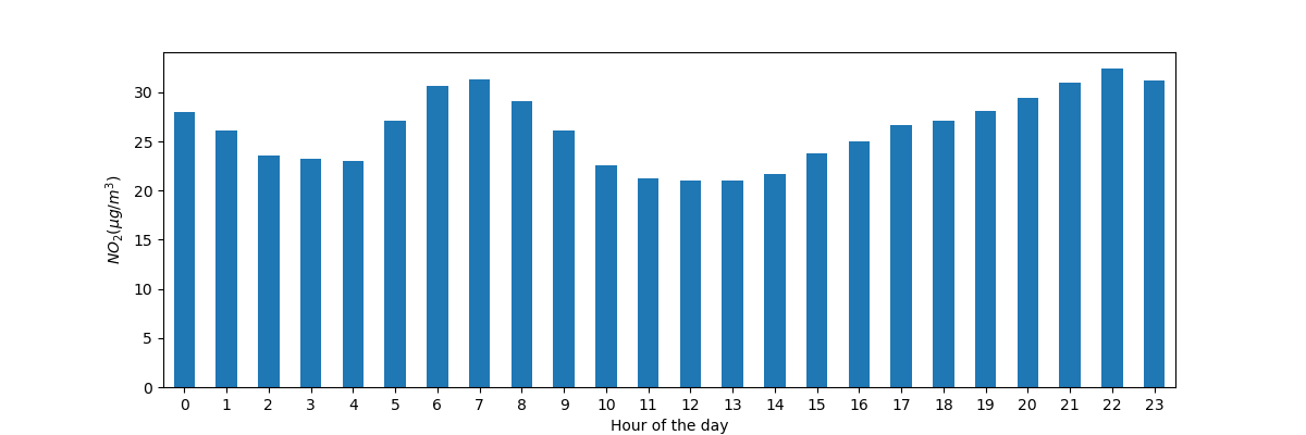
与上一个案例类似,我们希望计算给定统计量(例如平均 \(NO_2\))**对于一天中的每个小时**,并且我们可以再次使用“拆分-应用-合并”方法。对于这种情况,我们使用 pandas
Timestamp的日期时间属性hour,该属性也可以通过dt访问器访问。
日期时间作为索引#
在重塑教程中,介绍了 pivot() 用于重塑数据表,将每个测量位置作为单独的列
In [18]: no_2 = air_quality.pivot(index="datetime", columns="location", values="value")

In [19]: no_2.head()
Out[19]:
location                   BETR801  FR04014  London Westminster
datetime
2019-05-07 01:00:00+00:00     50.5     25.0                23.0
2019-05-07 02:00:00+00:00     45.0     27.7                19.0
2019-05-07 03:00:00+00:00      NaN     50.4                19.0
2019-05-07 04:00:00+00:00      NaN     61.9                16.0
2019-05-07 05:00:00+00:00      NaN     72.4                 NaN
注意
通过透视数据,日期时间信息成为表格的索引。通常,通过 set_index 函数可以将列设置为索引。
使用日期时间索引(即 DatetimeIndex)提供了强大的功能。例如,我们不需要 dt 访问器来获取时间序列属性,而是可以直接在索引上使用这些属性
In [20]: no_2.index.year, no_2.index.weekday
Out[20]:
(Index([2019, 2019, 2019, 2019, 2019, 2019, 2019, 2019, 2019, 2019,
        ...
        2019, 2019, 2019, 2019, 2019, 2019, 2019, 2019, 2019, 2019],
       dtype='int32', name='datetime', length=1033),
 Index([1, 1, 1, 1, 1, 1, 1, 1, 1, 1,
        ...
        3, 3, 3, 3, 3, 3, 3, 3, 3, 4],
       dtype='int32', name='datetime', length=1033))
其他一些优势包括方便的时间段子集选择或图表上调整的时间刻度。让我们将其应用于我们的数据。
绘制从 5 月 20 日到 5 月 21 日末不同站点的 \(NO_2\) 值图表
In [21]: no_2["2019-05-20":"2019-05-21"].plot();

通过提供一个**可解析为日期时间的字符串**,可以在
DatetimeIndex上选择数据的特定子集。
关于 DatetimeIndex 和使用字符串进行切片的更多信息,请参阅时间序列索引一节。
将时间序列重新采样到另一个频率#
将当前的每小时时间序列值聚合为每个站点的每月最大值。
In [22]: monthly_max = no_2.resample("ME").max()

In [23]: monthly_max
Out[23]:
location                   BETR801  FR04014  London Westminster
datetime
2019-05-31 00:00:00+00:00     74.5     97.0                97.0
2019-06-30 00:00:00+00:00     52.5     84.7                52.0
对带有日期时间索引的时间序列数据来说,一个非常强大的方法是能够将时间序列
resample()到另一个频率(例如,将秒级数据转换为 5 分钟级数据)。
resample() 方法类似于 groupby 操作
它通过使用定义目标频率的字符串(例如
M、5H等)提供基于时间的聚合它需要一个聚合函数,例如
mean、max等。
用于定义时间序列频率的别名概述在偏移别名概览表中给出。
定义后,时间序列的频率由 freq 属性提供
In [24]: monthly_max.index.freq
Out[24]: <MonthEnd>
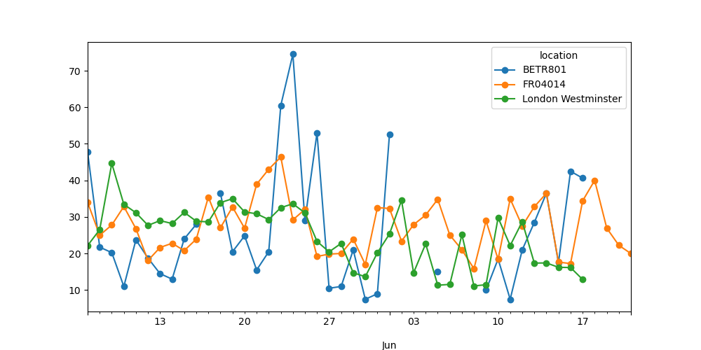
绘制每个站点的每日平均 \(NO_2\) 值图表。
In [25]: no_2.resample("D").mean().plot(style="-o", figsize=(10, 5));
关于时间序列 resampling 强大功能的更多详细信息在用户指南的重采样部分提供。
记住
有效的日期字符串可以使用
to_datetime函数或作为读取函数的一部分转换为日期时间对象。pandas 中的日期时间对象支持计算、逻辑操作以及使用
dt访问器访问的便捷日期相关属性。一个
DatetimeIndex包含这些日期相关属性并支持便捷的切片。Resample是一个强大的方法,用于改变时间序列的频率。
关于时间序列的完整概述,请参见时间序列和日期功能页面。